A beginners guide to Excel array formulas
This article explains the basics of array formulas, read this article if you never have used array formulas before. It opened up a new world to me and I am sure you will find many applications for these kinds of calculations.
What's on this webpage
- Why are array formulas so powerful?
- How to identify array formulas?
- How to enter an array formula?
- Why is only one value shown? I have x values in the array?
- What are vertical and horizontal arrays?
- How to use cell references in array formulas?
- How to quickly build an array
- How to hard code (literal) values in array formulas?
- Is Ctrl + Shift + Enter always necessary?
- Can I enter an array formula in merged cells?
- Are there any exceptions?
- Any caveats with array formulas?
- Alright, show me some useful array formulas?
- Excel 365 dynamic array formulas
- Get Excel file
- How to enter array formulas in merged cells
- How to use absolute and relative references
- Convert array formula to a regular formula
1. Why are array formulas so powerful?
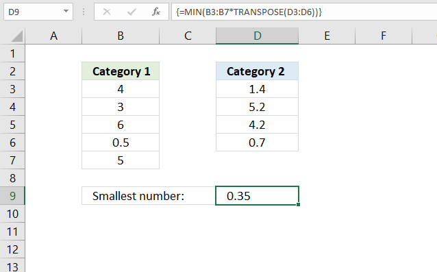
They allow you to do things not possible with regular formulas, an array formula can do multiple calculations based on several values simultaneously. You can do some seriously complicated calculations, Excel is definitively a powerful tool.
The array formula example, demonstrated in the image above, performs calculations to multiple numbers simultaneously and returns the smallest number from those calculations.
It multiplies all numbers in column B with all numbers in column D and returns the smallest product of all numbers.
Array formula in cell D9:
Explaining formula in cell D9
Step 1 - Transpose numbers
It is not possible to multiply two vertical arrays containing a different amount of numbers. The TRANSPOSE function converts a vertical array to horizontal and vice versa.
However, if they were of identical size the result would not be what we are looking for anyway, the first number would be multiplied with the first value in the second array only. We want each value multipled with all numbers in the second array to calculate all combinations.
TRANSPOSE(D3:D6)
becomes
TRANSPOSE({1.4;5.2;4.2;0.7})
and returns {1.4,5.2,4.2,0.7}.
Note that the delimiting character is a semicolon in the vertical array and a comma in the horizontal array.
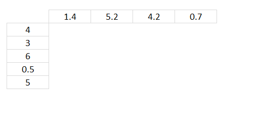
The image above shows the numbers in the second array arranged horizontally.
Step 2 - Multiply numbers
B3:B7*TRANSPOSE(D3:D6)
becomes
B3:B7*{1.4,5.2,4.2,0.7}
becomes
{4;3;6;0.5;5}*{1.4,5.2,4.2,0.7}
and returns {5.6,20.8,16.8,2.8;4.2,15.6,12.6,2.1;8.4,31.2,25.2,4.2;0.7,2.6,2.1,0.35;7,26,21,3.5}.
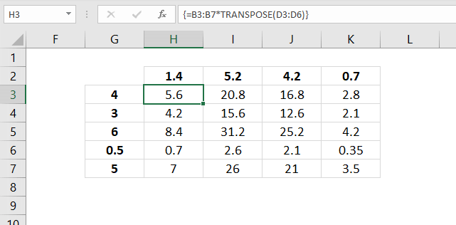
The result is shown in cell range H3:K7 in the image above. Cell H3 shows the product of the numbers in cell H2 and G3, and so on.
Step 3 - Extract the smallest number in the array
The MIN function returns the smallest number from a cell range or an array.
MIN(B3:B7*TRANSPOSE(D3:D6))
becomes
MIN({5.6,20.8,16.8,2.8;4.2,15.6,12.6,2.1;8.4,31.2,25.2,4.2;0.7,2.6,2.1,0.35;7,26,21,3.5})
and returns 0.35 which is the smallest number in the array.
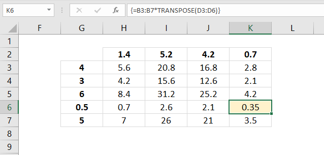
The image below shows the result in cell D9, all these calculations were completed in one cell only.

2. How to identify array formulas?
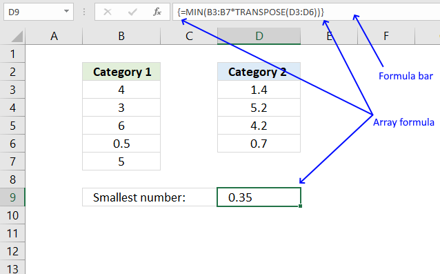
The formula bar is above your worksheet, it may be empty or contain a value or a formula. The image above demonstrates an array formula in cell D9.
The formula bar shows what kind of formula the selected cell contains. An array formula begins with a curly bracket and ends with a curly bracket.
These curly brackets appear automatically if you enter the formula as an array formula, see next section below on how to do that.
3. How to enter an array formula?
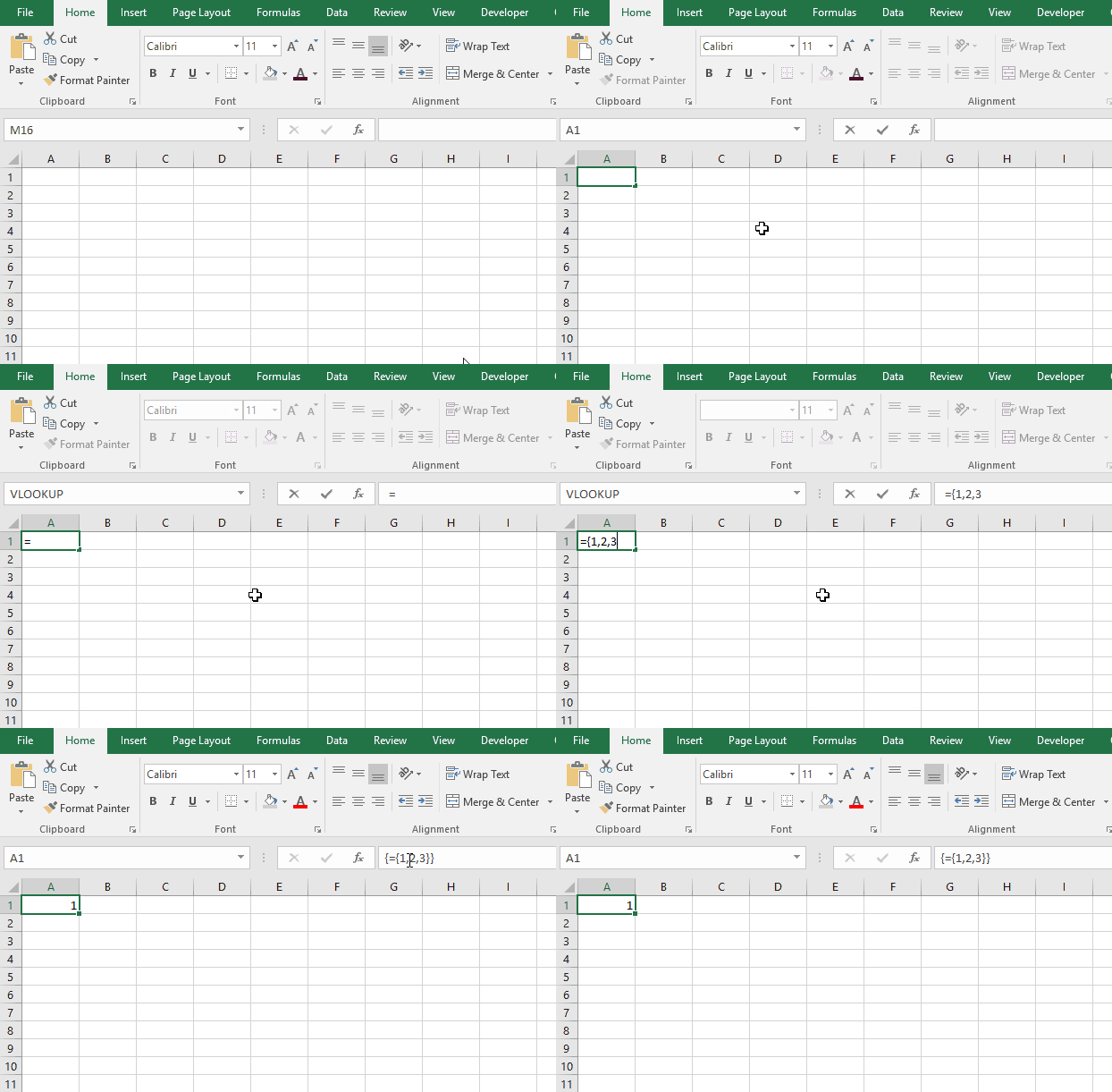
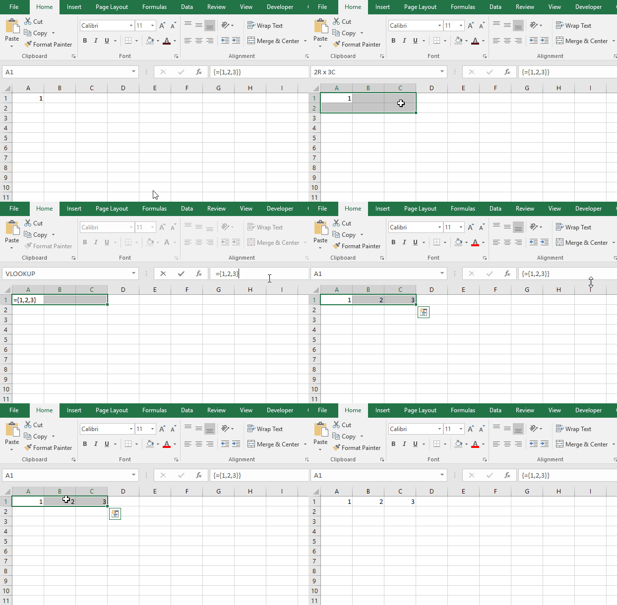
Constructing an array in Excel is easy. Double press with left mouse button on cell A1 and type ={1,2,3} in the formula bar and hold and press CTRL + SHIFT simultaneously, then press Enter once. Release all keys.
The formula in the formula bar now shows a beginning and ending curly bracket. Don't enter those characters yourself. Make sure the formula bar looks like this: {={1,2,3}}
If your formula bar looks like the picture above then you have made your first array! If not try again.
={1,2,3} is an array of constants separated by a delimiting character. This formula is entered in cell A1 but only one value in the array is displayed, why is that? The next section below explains why this happens.
4. Why is only one value shown? I have x values in the array?
There can only be one value in each cell. To be able to see all values enter the formula in cell range A1:C1
- Select cell range A1:C1
- Press with left mouse button on in the formula bar
- Press and hold CTRL + SHIFT simultaneously
- Press Enter
- Release all keys
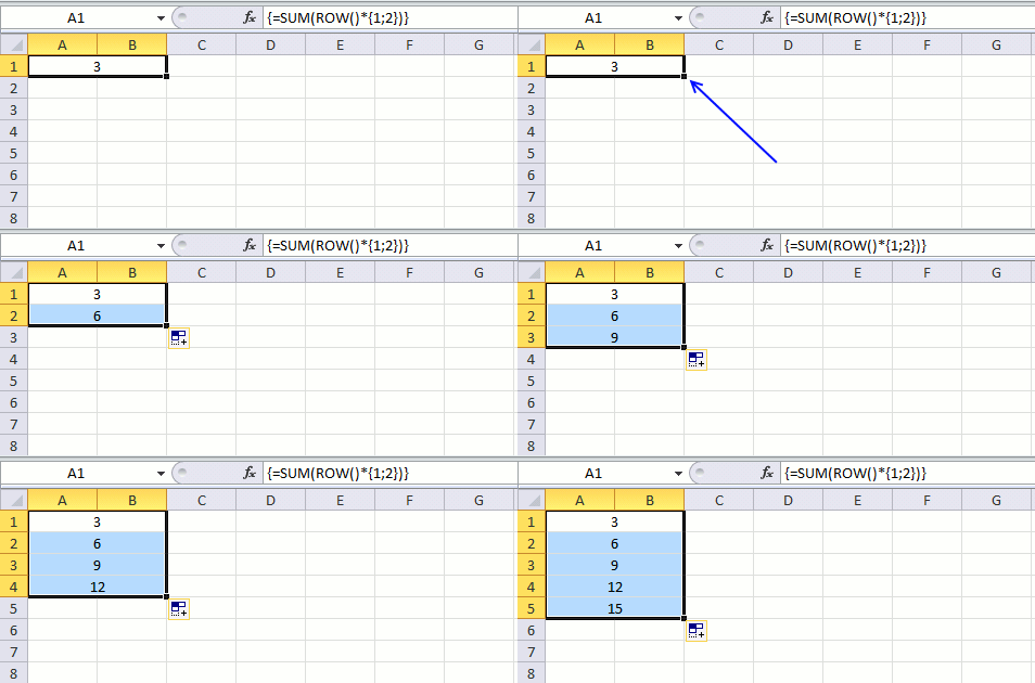
The animated picture above shows you how to extend an array formula from cell A1 to A1:C1, this allows you to see all values in the array.
You have now extended the formula to three cells and all values in the array are visible on the sheet, see picture above.
5. What are vertical and horizontal arrays?
You can construct arrays with a comma delimiter and a semicolon delimiter.
What is the difference? Use the comma when you want values horizontally and semicolon vertically. Look at the formula bar in this animated picture:
You can also combine colons and semicolons. ={1,2;3,4} A comma tells excel that the next value is to the right of the first value. A semicolon puts the next value on the next row.
I try to enter an array with text values but it doesn't work, why? Use double quotes around your values, like this: ={"A","B"}
6. How to use cell references in array formulas
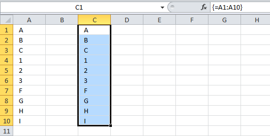
All arrays presented above contain constants, meaning they don't change unless you edit them. This formula =A1:A10 contains a cell reference to A1:A10. The values in this formula change if you change a value in cell range A1:A10. Formula =A1:A10 does not contain any constants.
This means that you can use values on your sheet in your array formula. This is extremely useful.
7. How to quickly build an array
I want to construct an array from 1 to 1000? I don't want to enter all these values.
You don't have to, the ROW function can do that for you. =ROW(1:1000) creates an array from 1 to 1000.
8. How to hard code (literal) values in array formulas?
Can I hard code values from 1 to 1000 in a formula without entering them myself? Yes, you can. Type =ROW(1:1000) in the formula bar and press F9.
Excel converts =ROW(1:1000) to ={1,2,3, ... , 1000)
9. Is Ctrl + Shift + Enter always necessary?
Can I build an array formula without entering it as an array formula?
Yes, you often can. However, it makes the formula more complicated.
Read this post: No more array formulas?
Excel 365 users enter array formulas as regular formulas, I recommend upgrading to Excel 365. There are so many new things in Excel 365.
10. Can I enter an array formula in merged cells?
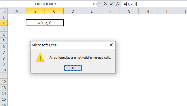
Excel tells me "Array formulas are not valid in merged cells", how can I enter array formulas in merged cells?
Yes, you can enter array formulas in merged cells using a workaround: How to enter array formulas in merged cells however, I recommend that you avoid merged cells as much as possible.
11. Are there any exceptions?
Yes, both the SUMPRODUCT function and the LOOKUP function lets you build arrays without requiring you to enter them as an array formula.
Recommended articles
The SUMPRODUCT function calculates the product of corresponding values and then returns the sum of each multiplication.
Recommended articles
Finds a value in a sorted cell range and returns a value on the same row.
The INDEX function lets you encapsulate an array so you don't need to enter it as an array formula:
Recommended articles
This article explains how to avoid array formulas if needed. It won't work with all array formulas, however, smaller ones […]
Recommended articles
Gets a value in a specific cell range based on a row and column number.
12. Any caveats using array formulas?
A major disadvantage with array formulas is that if you double press with left mouse button on a cell containing an array formula and then press with left mouse button on another cell, the array formula changes to a regular formula. Beginner Excel users may not know about this and could possibly break your worksheet calculations.
However, this is not the case if you press the Escape key to exit editing an array formula or if you press CTRL + SHIFT + Enter.
Array formulas can slow down your worksheet calculations.
13. Alright, show me some useful array formulas?
Recommended articles
First, let me explain the difference between unique values and unique distinct values, it is important you know the difference […]
Recommended articles
This post explains how to lookup a value and return multiple values. No array formula required.
Recommended articles
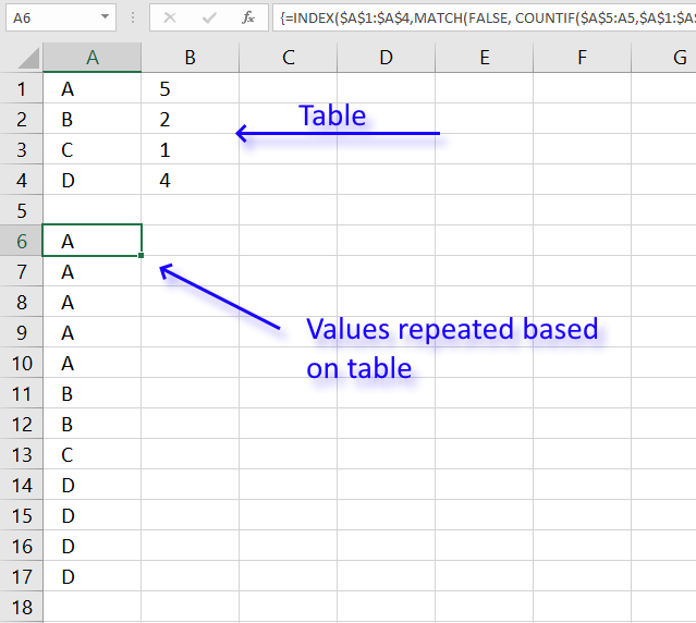
Table of Contents Repeat values Repeat the range according to criteria in loop Find the most/least consecutive repeated value […]
Cool, even more complicated calculations?
Recommended articles
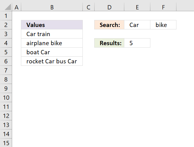
This article demonstrates an array formula that counts how many times multiple text strings exist in a cell range. The […]
Recommended articles
This article demonstrates a scoreboard, displayed to the left, that sorts contestants based on total scores and refreshes instantly each […]
Recommended articles
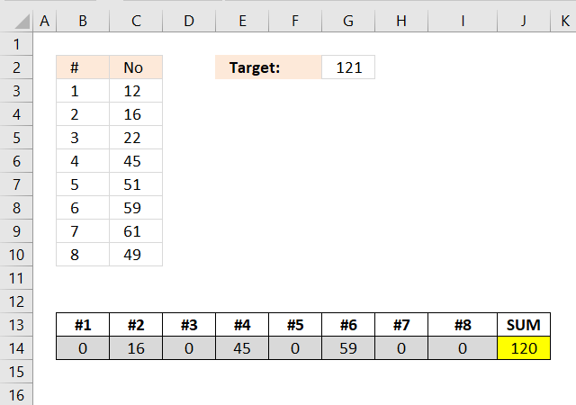
Excelxor is such a great website for inspiration, I am really impressed by this post Which numbers add up to […]
Recommended articles
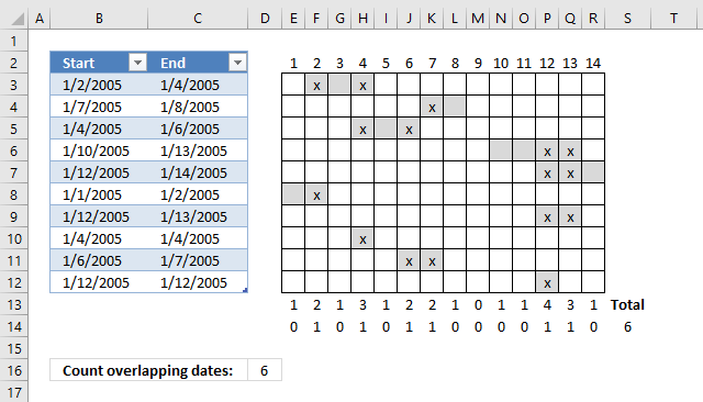
This post demonstrates a formula in cell D16 that counts overlapping dates across multiple date ranges. The date ranges are […]
14. Excel 365 dynamic array formulas
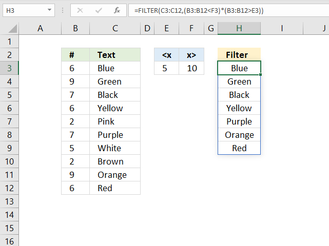
You can enter array formulas in Excel 365, however, there is no need to do that. Microsoft has now changed how array formulas are entered, they are entered as a regular formula and are now called dynamic array formulas.
Excel 365 shows all values that the array formula returns automatically if the array formula returns more than one value, this behavior is called spilling.
The image above shows a dynamic array formula in cell H3 that returns multiple values and spills those values to cells below. The FILTER function is a new function only available for Excel 365 users.
16. How to enter array formulas in merged cells
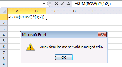
Have you ever tried to enter an array formula in merged cells? Then you are familiar with this error message: Array formulas are not valid in merged cells.
This is not true, they can be entered in merged cells.
Here are a few suggestions to solve this problem.
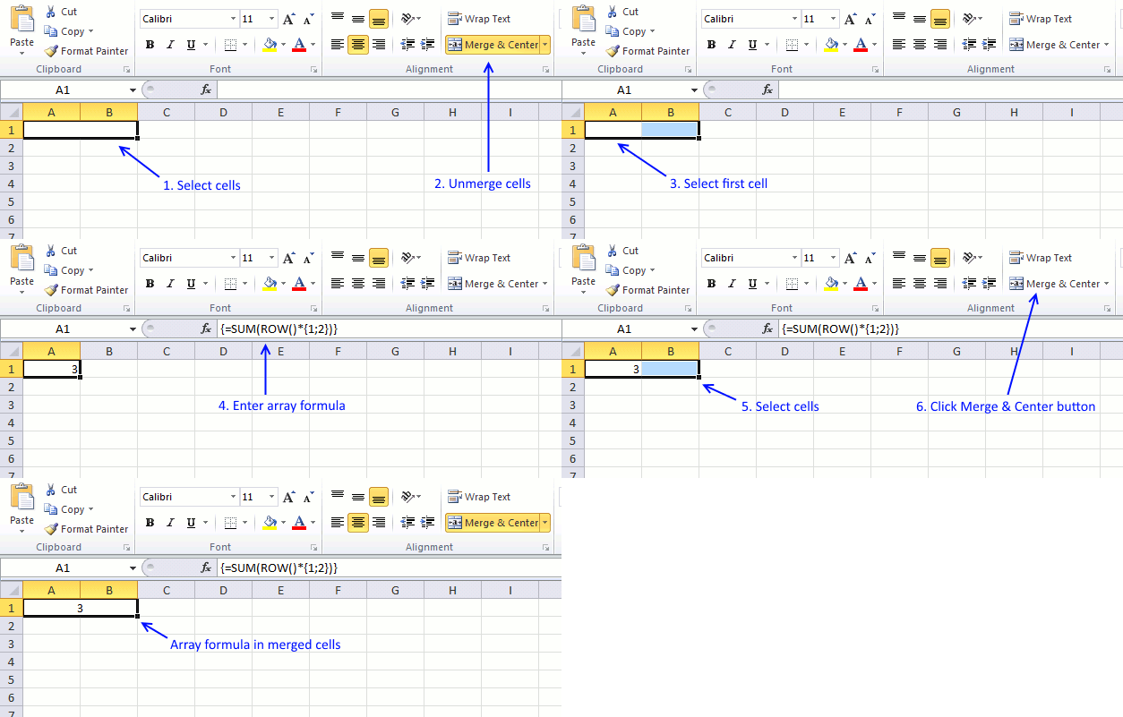
16.1 Unmerge cells
- Select the merged cell.
- Go to tab "Home" on the ribbon.
- Press with left mouse button on the "Merge & Center" button to unmerge cells.
- Select the first cell of the unmerged cell.
- Enter the array formula.
- Select the cells you want to merge.
- Press with left mouse button on the "Merge & Center" button to merge cells.
Tip! You don't need to repeat these actions for all cells below, just press and hold on the black dot on the lower right corner of the cell, then drag down as far as needed. See animated image below.
16.2 Excel defined named ranges
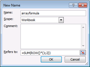
This workaround requires you to create a named range containing the array formula you want to use. Here are the steps.
- Go to tab "Formula" on the ribbon.
- Press with left mouse button on "Name Manager".
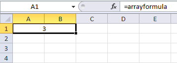
- Type a name, I named it arrayformula.
- Enter the array formula in "Refers to:" field.
- Press with left mouse button on OK button.
- Select the merged cell.
- Type =arrayformula
- Press enter.
16.3 Excel 365 dynamic array formulas and merged cells?
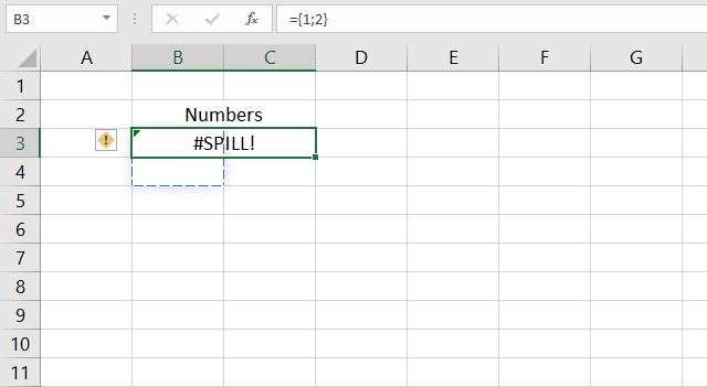
The image above shows what happens when you try to enter a dynamic array formula in a merged cell in Excel 365.
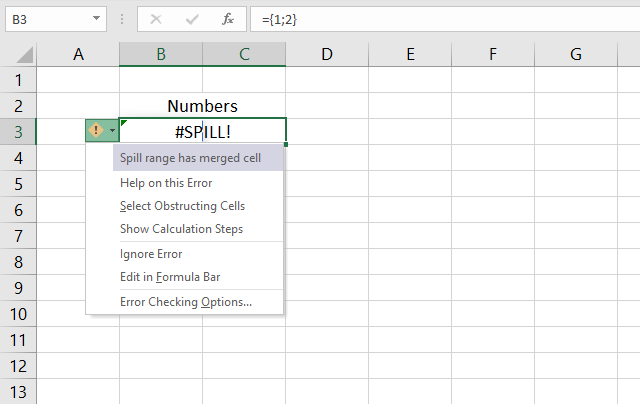
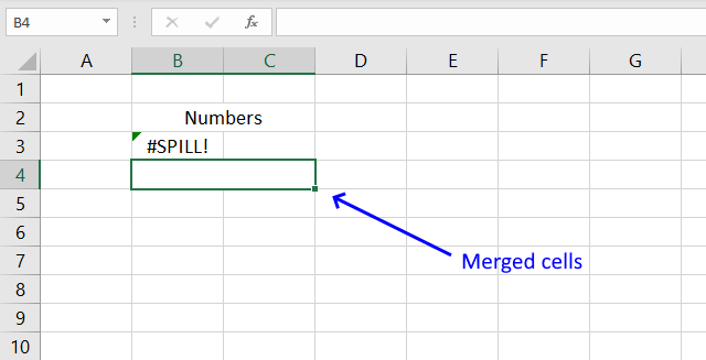
Merged cells don't work with Excel 365 dynamic array formulas, the #SPILL error is what you get if you try to enter the formula in a merged cell or if a merged cell is in the spilling range.
17. How to use absolute and relative references
What is a reference in Excel? Excel has an A1 reference style meaning columns are named letters A to XFD and rows have numbers, 1 to 1 048 576. The total number of columns in Excel 2007 are 16384.
A cell can contain a value, formula or constants. A formula starts with a = (equal) sign. You can use values from other cells in your formula. To use another value you create a reference to the cell containing the value you want to use in your formula.
A formula starts with a "=" equal sign. A reference is a column letter and a row number, like B1. B is the column B and 1 is row number one.
Example:
- Double press with left mouse button on cell A1 and type =B1 then press Enter
- Double press with left mouse button on cell B1 and type 11 then press Enter
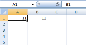
You have now created a reference to cell B1. B1 contains the value 11. A1 contains the reference to B1 so both cells now show the number 11. Excel uses relative references by default. =B1 is a relative reference.
17.1 What is a relative reference in excel?
When you copy a cell containing a relative reference and paste it into another cell, the relative reference changes. Let me show you an example.
Now copy cell A1 and paste it to cell A3.
- Press with right mouse button on on cell A1 and press with left mouse button on Copy
- Press with right mouse button on on cell A3 and press with left mouse button on Paste
- Press Escape to remove selection.
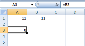
When you copy a formula containing relative references the reference changes when you paste it into a another cell. Select cell A3. The formula window now show =B3. See picture above.
Cell A3 has the value 0 (zero) and the formula field shows the relative reference =B3. Cell B3 is empty and that is why cell A3 displays 0 (zero).
When you copied the cell reference in cell A1 to A3, the relative reference changed to B3. The reference changed two rows down. The exact same number as of rows between the copied cell A1 and cell A3.
How much the reference changes is relative to the position of the copied cell and the position of the new cell the formula is pasted into. Excel uses relative references by default.
17.2 How to change a relative reference to an absolute reference.
- Double press with left mouse button on A1.
- Press F4
- Press Enter
The relative reference =B1 changes to an absolute reference =$B$1.
17.3 What is an absolute reference in excel?
An absolute reference in a formula stays the same if copied to another cell.
Example:
- Press with right mouse button on cell A1 and press with left mouse button on Copy
- Press with right mouse button on cell A3 and press with left mouse button on Paste
- Press Escape to remove selection.
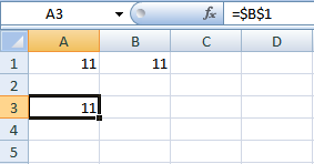
Select cell A3
The cell reference in cell A3 stays the same (is locked to cell B1). An absolute reference does not change when copied or filled into other cells.
17.4 Insert a row or column
Remember, if you insert a row or column into your excel sheet the absolute reference changes.
Example
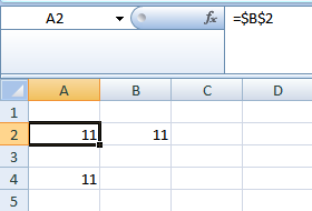
Cell A1 contains an absolute reference to B1 (=$B$1).
The absolute reference changed to =$B$2.
To keep absolute references use INDIRECT function.
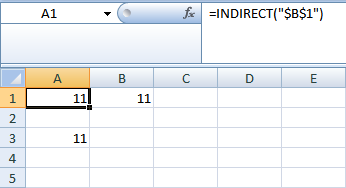
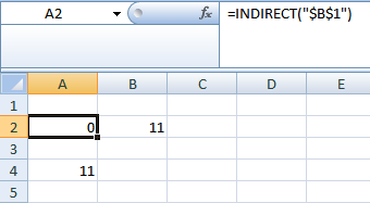
- Type =INDIRECT("$B$1") + ENTER in cell A1
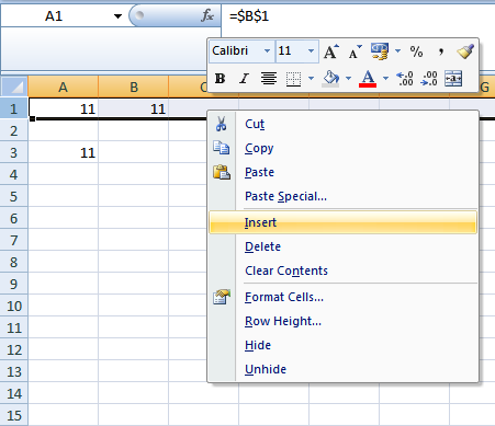
- Select row 1
- Press with right mouse button on on row 1 and select "Insert"
- Done!
The absolute reference is still referencing $B$1. $B$1 is empty and $B$1 returns a 0 (zero).
There is a downside using INDIRECT. INDIRECT is a volatile function. A volatile function is recalculated every time a recalculation is made. You might think that is alright. But if your excel sheet has many calculations and INDIRECT is often used, the calculation can become very slow.
18. Convert array formula to a regular formula
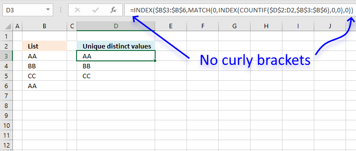
This article explains how to avoid array formulas if needed. It won't work with all array formulas, however, smaller ones seem fine.
Important! Excel 365 uses dynamic array formulas which are entered as regular formulas simply by pressing Enter. A dynamic array formula spills values to cells below and to the right as far as needed.
You can ignore this article entirely if you use Excel 365.
Dynamic array formulas have these characteristics:
- Work exactly the same as regular array formulas.
- Easier to enter.
- Expand to cells below automatically.
- Don't break as easily as regular array formulas.
- Adjacent cells below and to the right must be empty or a spilling error appears: #SPILL!.
Why would you want to avoid array formulas? An inexperienced Excel user may turn it into a regular formula by editing it and then press Enter. That will break the array formula, and often but not always, an error will be returned.
Now, if you can't avoid an array formula, you could lock the cell containing the array formula and protect the worksheet. I will explain how to do this, as well.
The following conversation inspired me to write this article.
CSE is an abbreviation for CTRL + SHIFT + ENTER, which is how you enter an array formula.
Kamran Mumtaz: This is the formula given by Aladin Akyurek without (CSE)...
This formula is exciting, I have never seen this approach before. It looks like an array formula, but it is not. It opens up possibilities that I have not thought about before.
Example 1,
This formula derives from the following article: Extract a unique distinct list
The original array formula:
The new regular formula in cell B2:
The new formula is NOT an array formula! Amazing! I am not sure if all array formulas can be converted to regular formulas, but some can.
Update: I am now using an even smaller regular formula that is not using this method at all. The LOOKUP function can do things that would generally require an array formula. See this article for more: Extract a unique distinct list
Explaining formula in cell B2
The formula in column B extracts unique distinct values from column A without the need to create an array formula.
I will explain below the calculation steps and the workaround that makes this possible.
Step 1 - Count cells based on condition(s)
The COUNTIF function counts cells in a cell range based on a condition. COUNTIF(range, criteria), range is $B$1:B1 and criteria is $A$2:$A$5.
This seems perhaps wrong, but it is not. $ B$1:B1 is a cell reference that expands when the cell is copied and pasted to cells below. The dollar signs in $B$1 make this part of the cell ref absolute, meaning it is locked.
The other part is B1, and that cell ref is relative, meaning it changes from cell to cell, for this to work you need to copy the cell and not the formula.
COUNTIF($B$1:B1,$A$2:$A$5)
becomes
COUNTIF("Unique distinct values", {"AA";"BB";"CC";"AA"})
and returns {0; 0; 0; 0}.
This means that "Unique distinct values" is not equal to any value in this array {"AA";"BB";"CC";"AA"}. This method requires you usually to enter the formula as an array formula. However, the next step is a workaround.
Step 2 - Create a regular formula
Generally, If the COUNTIF function returns an array, this would require you to enter the formula as an array formula. However, if you encapsulate the COUNTIF function with the INDEX function you can create a workaround. Unfortunately it comes with a cost, the formula grows larger.
INDEX(COUNTIF($B$1:B1,$A$2:$A$5),0,0)
returns {0; 0; 0; 0}.
You can shorten the INDEX function to
INDEX(COUNTIF($B$1:B1,$A$2:$A$5),)
and the result will be the same.
Step 3 - Find first value not displayed
The MATCH function returns the relative position of the first value that is equal to 0 (zero). MATCH(lookup_value, lookup_array, [match_type])
MATCH(0,INDEX(COUNTIF($B$1:B1,$A$2:$A$5),0,0),0)
becomes
MATCH(0,{0; 0; 0; 0},0)
and returns 1. 0 (zero) is equal to the first value in the array.
Step 4 - Return value based on row number
The INDEX function returns a value from a given cell range based on a specified row number. INDEX(array, [row_num], [column_num])
INDEX($A$2:$A$5, MATCH(0, INDEX(COUNTIF($B$1:B1, $A$2:$A$5), 0, 0), 0))
becomes
INDEX($A$2:$A$5, 1)
and returns "AA" in cell B2.
Example 2,
This example comes from this article: How to return multiple values using vlookup. The formula returns values based ona condition, if value in cell E1 is equal to one or many values in cell range A2:A5 the formula will return the corresponding values from B2:B5.
Original array formula:
The new regular formula in cell E2:
Explaining formula in cell E2
Step 1 - Compare values
The equal sign lets you check if a value is equal to another value or multiple values.
$A$2:$A$5=$E$1
returns {TRUE; FALSE; FALSE; TRUE}.
Step 2 - Create an array of numbers from 1 to n
We need an array of numbers starting from 1 to n where n is the total number of rows in the cell range.
MATCH(ROW($B$2:$B$5), ROW($B$2:$B$5))
returns {1;2;3;4}. There are four rows in cell range $B$2:$B$5.
Step 3 - Multiply logical expression with array
The asterisk character allows you to multiply numbers, arrays, and constants in a formula. Use parentheses to control the order of operation.
($A$2:$A$5=$E$1)*(MATCH(ROW($B$2:$B$5), ROW($B$2:$B$5)))
returns {1;0;0;4}.
TRUE and FALSE are boolean values, their numerical equivalents are 1 and 0 (zero). For example TRUE*1=1, FALSE*1=0.
Step 4 - Check if values are not equal to value in E1
This step contains a logical expression that returns TRUE if a value is not equal to cell E1 and FALSE if equal. Combine a less than and greater than character to check if values are not equal.
$A$2:$A$5<>$E$1
returns {FALSE; TRUE; TRUE; FALSE}.
Step 5 - Multiply with a value greater than the maximum row number
A worksheet can contain up to 1048576 rows, a larger number will return an error in step 9.
($A$2:$A$5<>$E$1)*1048577
returns {0; 1048577; 1048577; 0}
Step 6 - Add arrays
The plus sign + lets you add arrays.
($A$2:$A$5=$E$1)*(MATCH(ROW($B$2:$B$5), ROW($B$2:$B$5)))+($A$2:$A$5<>$E$1)*1048577
returns {1; 1048577; 1048577; 4}
Step 7 - Remove need for array formula
The INDEX function lets you do calculations without requiring you to create an array formula.
INDEX(($A$2:$A$5=$E$1)*(MATCH(ROW($B$2:$B$5), ROW($B$2:$B$5)))+($A$2:$A$5<>$E$1)*1048577, 0, 0)
returns {1; 1048577; 1048577; 4}
Step 8 - Extract k-th smallest number in array
The SMALL function extracts the k-th smallest number in the array, this step makes sure that different values display in every cell.
SMALL(INDEX(($A$2:$A$5=$E$1)*(MATCH(ROW($B$2:$B$5), ROW($B$2:$B$5)))+($A$2:$A$5<>$E$1)*1048577, 0, 0), ROW(A1))
returns 1.
Step 9 - Return value from cell range
This step utilizes the INDEX function to fetch a value from cell range B2:B5.
INDEX($B$2:$B$5, SMALL(INDEX(($A$2:$A$5=$E$1)*(MATCH(ROW($B$2:$B$5), ROW($B$2:$B$5)))+($A$2:$A$5<>$E$1)*1048577, 0, 0), ROW(A1)))
returns 1 in cell E2.
The IF function has a logical expression that compares multiple values to a condition.
How to lock cells
You can lock cells so they can't be edited and that would make it safer to use array formulas. Keep in mind that there are tools out there that can open up password-protected sheets easily.
All cells in a worksheet are locked by default, you can verify this. Select any cell in your worksheet, press CTRL + 1 to format cell. Go to tab "Protection".
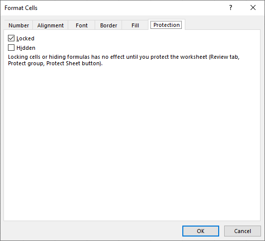
This tab shows you if the cell is locked, the checkbox is enabled if it is locked. To lock cells you need to protect the worksheet.
- Go to the worksheet you want to protect.
- Go to tab "Review" on the ribbon.
- Press with mouse on "Protect sheet" button.
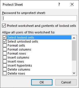
- Enter a password you want to use. Remember it because you will need it next time you want to unprotect the worksheet.
- Press with left mouse button on OK button.
What do you prefer? Array formulas or somewhat longer and more complicated regular formulas?
Arrays category
This post will teach you how to work with Excel arrays in visual basic for applications (VBA). Why do you […]
Excel categories
19 Responses to “A beginners guide to Excel array formulas”
Leave a Reply
How to comment
How to add a formula to your comment
<code>Insert your formula here.</code>
Convert less than and larger than signs
Use html character entities instead of less than and larger than signs.
< becomes < and > becomes >
How to add VBA code to your comment
[vb 1="vbnet" language=","]
Put your VBA code here.
[/vb]
How to add a picture to your comment:
Upload picture to postimage.org or imgur
Paste image link to your comment.













[...] D25:$D$25 is a relative and absolute cell reference. [...]
Interesting Formula, but if the purpose is to avoid the CSE, and its Excel2010, then this is far simpler formula:
=INDEX(Price,AGGREGATE(15,6,(ROW(Product)-MIN(ROW(Product))+1)/(Product=$E$1),ROW(A1)))
No CSE required.
chrisham,
Great comment! From now on, I am going to provide both array formulas and regular formulas. I am going to let the reader decide which formula to use.
I´ll also update the most read posts with their equivalent formulas.
Wow.. nice.. I HATE array formulas..
It doesnt work with multiple columns so I daisy chained them together sorting A1:A6 and putting the result in C1:C6. Then sort B1:B12 and put the result in C7:C19.
Now sort C1:C19 and put the results in D1:D19...
If you dont like the #N/A, =IFERROR() will get change them to something more palatable.
Awesome.. thanks guys!!
One more comment.. this is a very processor intensive formula. I used it for a thousand cells (just pulled it down) and it takes +4 minutes to open the spread sheet and will often crash.
I narrowed down the problem to the formula and just use it on 120 cells the spreadsheet opens quickly and calculates/recalculates quickly.
Thanks again guys!
JL
Jeff,
Yes, array formulas can be cpu intensive.
[...] can enter a reference to a single cell or a cell range. The ROW function returns an array of numbers if you enter a [...]
HOW TO AUTO SEARCH NAME THE DISPLAY
LALIT,
CAN YOU EXPLAIN IN GREATER DETAIL?
[…] There are relative cell references in the CONCATENATE function and they change in each cell. Don´t know much about relative and absolute cell references? Read this: Absolute and relative references in excel […]
Oscar,
This "non-array" formula concept may be of some benefit after all. I had been working on making workbooks to load into Office on Windows Phone 8 that would be tailored for our field personnel. Only to find that Excel in Office for Windows Phone does NOT support array formulas (among other things).
By modifying the examples Chrisham used, it has proven to be a worthwhile endeavor. I'd be interested in other examples should any be out there.
Thanks and regards,
Leroy
First, this is the greatest site I ever found regarding excel tips and tricks and the way you explain your solutions!! My question: I have noticed that array formulas are very calculation intensive, so when you have 500 or more lines, calculating the sheet gets slow. What is your experience or recommendation regarding the size limits of using array formulas efficiently? I did not find anything posted... (I work with sheets that have tens of thousands of lines)
[…] Diagramme wirken mitunter überladen und sind deshalb schwer zu deuten. Autor Alexander Wildt zeigt, wie mit Hilfe von Steuerelementen Säulendiagramme in verschiedenen Perspektiven dargestellt werden können. Get-Digital-Help 07.09.2015 „Learn the basics of Excel arrays“ https://www.get-digital-help.com/learn-the-basics-of-excel-arrays/ […]
I liked this formula so I could get a list of items, but then do a calculation on the resulting list. I also wanted the original list to be of any length, and so I wouldn't know the length of the resultant list. With the #N/A error, this means I would have to go back and manually adjust the length of the final list (because the #N/A would mess up the calculations.
I adapted the above formula to replace any #N/As with blanks:
=IF(ISERROR(INDEX($A$2:$A$11,MATCH(0,INDEX(COUNTIF($B$1:B1,$A$2:$A$11),0,0),0))),"",INDEX($A$2:$A$11,MATCH(0,INDEX(COUNTIF($B$1:B1,$A$2:$A$11),0,0),0)))
It's sort of clunky, but it worked for me. The double quotes could be replaced with whatever filler you would need in case your calculations call for it...
[…] formula is valid for cell A3, when you copy it to cell A4 the cell refs change. Check out blog post absolute and relative cell references and learn how to build smarter […]
Hi Oscar,
Greetings. I was trying using the ARRAY Formula in the merged Cell, but facing an issue.
For a simple formula in the merged cell, the formula as explained on the website works perfectly but when I try to use it in another merged cell which contains HYPERLINK, I get #REF. I have pasted the code here for your reference. if you could please let me know what is wrong in this code.
=HYPERLINK(INDEX('01-08-2011'!$C$4:$L$129,MATCH(SEARCH!$C$2,'01-08-2011'!$C$4:$C$1159,0),11))
Thanks and regards,
Ali.
Done... Its Resolved :D
Thanks and regards,
Ali.
[…] formula basics in conditional formatting. It is really good if you have some knowledge about absolute and relative cell references but it is not necessary. I think the examples shown here explains a lot when it comes to cell […]
Hi Oscar
I tried your example as above, but it does not function on my spreedsheet.
=INDEX($C$3:$C$7, SMALL(IF(($B$10=$B$3:$B$7), MATCH(ROW($B$3:$B$7), ROW($B$3:$B$7)), ""),ROWS($A$1:A1)))Please assist.
PS. I'm using MS Offic 2010
Regards
Leslie