Wildcard lookups and include or exclude criteria
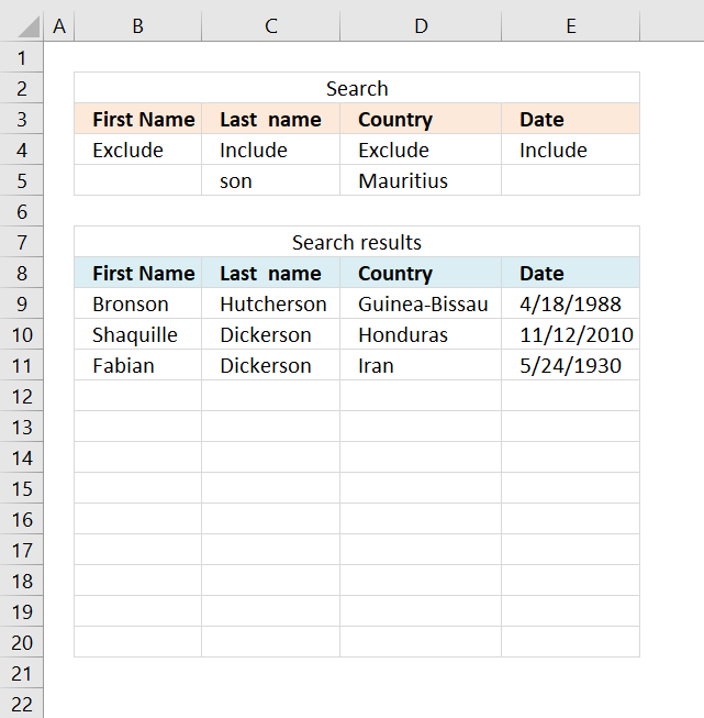
This article demonstrates three different ways to filter a data set if a value contains a specific string and if a cell is not equal (exclude) to a specific value. The image above shows an array formula in cell range B9:E20 that extracts values based on the conditions on row 5 and the drop-down lists on row 4.
What's on this page
1. Question
Hi Oscar,
This is great and compliments your Multiple Criteria and Multiple Matches series of posts very well. However, I have been trying to modify the array formulas in the 3rd and 4th posts of that series to cope with wildcard searches or part cell matches and thought this post may help but not so far, unfortunately.
I have tried numerous approaches but can't seem to get a multiple criteria series of "searches" (or counts) to work with anything but exact data.
I'm trying to search for part of a serial number e.g.(A110 within a string A110E12694369020 as one of my search inputs. In this case, it is always the first 4 digits but I'd like to be able to input just A1 or *A1* into a search cell and not rely on reviewing the first 4 characters as this is not always the result for these serial numbers.
I'm also looking for items with corresponding dates equal or before a certain due date search string - your 4th post to Lookup-with-multiple-criteria-and-display-multiple-search-results-using-excel-formula-part-4-john helped me resolve these criteria though.
Finally, I'm trying another 'wildcard' search and to find FSS (or *FSS*) OR the exact inverse of this - so NOT containing FSS (or *FSS*) - and both of these search criteria are proving elusive to me.
All the data I have is in a large table but I'm not sure if I can alter it to be an Excel Table (which might help), as it is in a sheet that is deleted and replaced by an irregular macro from another workbook and this may corrupt a Table setup(?). It can not be a Pivot as the data is in a shared workbook and Pivot Tables do not update when in shared documents - hence the Array solution I am trying to develop. I have successfully named the columns of ranges I need though without losing them on an update of data.
To summarise - I'd like to search by some form of a wildcard; *app* to return a positive result for "apple" and to search for the opposite; have criteria that would exclude "apple" using something like *app*
Although I have around 80 columns I'm just looking to return the serial number in say Column A based on these multiple criteria; Col B <= a date, Col C does NOT contain a wildcard string *whatever*, Col D DOES contain a different wildcard string, Col E EXACTLY equals a third search string etc. I am happy to build up the criteria for more columns beyond this if I can resolve the NOT and the wildcard elements.
I'd really appreciate some further pointers, thanks Oscar!
2. Wildcard lookups and include or exclude criteria - Excel 365
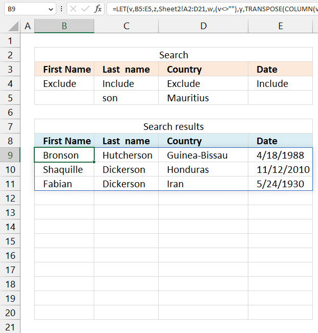
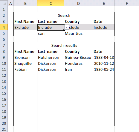
The image above shows an Excel 365 formula that extracts records from a data set located on sheet2 based on criteria specified in cells B3:E5. Cells B4:E4 allow you to include or exclude specific conditions using drop down lists. A missing condition (blank) in cells B5:E5 is not used into the calculation, in other words, it is ignored.
Note that the formula looks for partial matches meaning a match is found if a string is found somewhere in the value. For example, string "pp" is found in value "apple" but not in "banana". An "excluded" string means that the cell can't contain (partial match) the given condition.
Excel 365 dynamic array formula in cell B9:
The formula in cell B9 spills values to cell B9 and adjacent cells below and to the right as far as needed. A #SPILL! error indicates that the spill range is not empty. Clear the destination cells and the error will go away. An Excel 365 dynamic array formula is different from legacy array formulas. Simply press Enter to after typing or copy/paste the formula to a given cell.
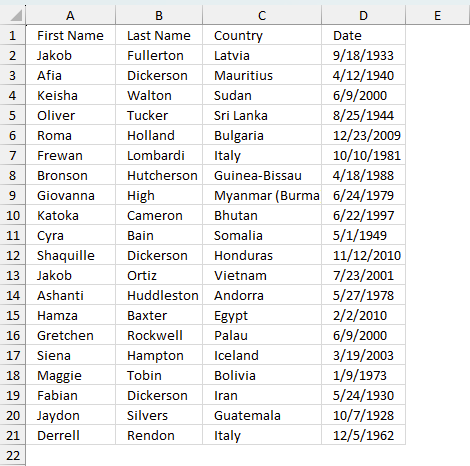
Sheet2 contains the source data displayed in the image above.
Explaining formula in cell B9
I recommend using the "Evaluate Formula" tool located on tab "Formula" on the ribbon. Press with left mouse button on the "Evaluate Formula" button to start the tool, a dialog box appears.
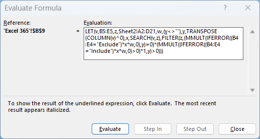
- Reference shows the cell reference that is being evaluated.
- Evaluation shows the formula. An underlined expression is what will be processed if you press with left mouse button on the "Evaluate" button. An italicized value is the most recent result.
- Press with left mouse button on the "Evaluate" button repeatedly to iterate through all expressions or intermediate calculations in the formula. The last result always matches the displayed cell value.
- Press with left mouse button on the "Close" button to dismiss the dialog box.
Step 1 - Check if cells in row 4 equal "Include"
The equal sign lets you compare value to value, it also compares a value to multiple values returning an array of boolean values TRUE or FALSE.
B4:E4="Include"
returns {TRUE, FALSE, TRUE, FALSE}
Step 2 - Check if cell range A2:D21 contains any of the values in B5:E5
The SEARCH function returns the number of the character at which a specific character or text string is found reading left to right (not case-sensitive)
Function syntax: SEARCH(find_text,within_text, [start_num])
SEARCH(B5:E5,Sheet2!A2:D21)
returns {1,#VALUE!,#VALUE!,1;1,7, ... ,1}
The SEARCH function returns a number corresponding to the position of the found string, an error is returned if not found.
Step 3 - Check if cells B5:E5are not empty
The less than and greater than signs lets you check if a value is not equal to another value. The result is a boolean value TRUE or FALSE.
B5:E5<>""
becomes
{"","son","Mauritius",""}<>""
and returns
{FALSE,TRUE,TRUE,FALSE}
Step 4 - Multiply arrays
The asterisk lets you multiply numbers and/or boolean values in an Excel formula, it works also with arrays.
This performs AND logic between two boolean values.
TRUE * TRUE = TRUE
TRUE * FALSE = FALSE
FALSE * TRUE = FALSE
FALSE * FALSE = FALSE
TRUE and FALSE are converted to their numerical equivalents:
TRUE - 1
FALSE - 0 (zero)
(B4:E4="Include")*SEARCH(B5:E5,Sheet2!A2:D21)*(B5:E5<>"")
returns {0,#VALUE!,#VALUE!,0;0,0, ... ,0}
Step 5 - Remove errors and replace them with 0 (zero)
The IFERROR function if the value argument returns an error, the value_if_error argument is used. If the value argument does NOT return an error, the IFERROR function returns the value argument.
Function syntax: IFERROR(value, value_if_error)
IFERROR((B4:E4="Include")*SEARCH(B5:E5,Sheet2!A2:D21)*(B5:E5<>""),0)
returns {0, 0, 0, 0; 0, 0, ... , 0}.
Step 6 - Check if valie is larger than 0 (zero)
IFERROR((B4:E4="Include")*SEARCH(B5:E5,Sheet2!A2:D21)*(B5:E5<>""),0)>0
returns {FALSE, FALSE, ... , FALSE}.
Step 7 - Convert boolean values to numerical values
The MMULT function can't work with boolean values, however, their numerical equivalents are fine.
(IFERROR((B4:E4="Include")*SEARCH(B5:E5,Sheet2!A2:D21)*(B5:E5<>""),0)>0)*1
returns {0, 0, 0, 0; 0, 0, ... , 0}
Step 8 - Calculate column numbers
The COLUMN function returns the column number of the top-left cell of a cell reference.
Function syntax: COLUMN(reference)
COLUMN(B5:E5)
returns
{2,3,4,5}
Step 9 - Convert numbers to 1
COLUMN(B5:E5)^0
becomes
{2,3,4,5}^0
and returns
{1,1,1,1}
Step 10 - Rearrange values
The TRANSPOSE function converts a vertical range to a horizontal range, or vice versa.
Function syntax: TRANSPOSE(array)
TRANSPOSE(COLUMN(B5:E5)^0)
returns {1; 1; 1; 1}
Step 11 - Sum numbers in array row-wise
The MMULT function calculates the matrix product of two arrays, an array as the same number of rows as array1 and columns as array2.
Function syntax: MMULT(array1, array2)
MMULT((IFERROR((B4:E4="Include")*SEARCH(B5:E5,Sheet2!A2:D21)*(B5:E5<>""),0)>0)*1,TRANSPOSE(COLUMN(B5:E5)^0))
returns {0; 1; 0; 0; 0; 0; 1; 0; 0; 0; 1; 0; 0; 0; 0; 0; 0; 1; 0; 0}
Step 12 - Check i cells equals "Exclude"
The equal sign lets you compare value to value, it also compares a value to multiple values returning an array of boolean values TRUE or FALSE.
B4:E4="Exclude"
returns {TRUE, FALSE, TRUE, FALSE}.
Step 13 - Check if numbers in array are equal to 0 (zero)
The MMULT function calculates the matrix product of two arrays, an array as the same number of rows as array1 and columns as array2.
Function syntax: MMULT(array1, array2)
MMULT(IFERROR((B4:E4="Exclude")*SEARCH(B5:E5,Sheet2!A2:D21)*(B5:E5<>""),0),TRANSPOSE(COLUMN(B5:E5)^0))=0
returns {TRUE; FALSE; ... ; TRUE}.
Step 14 - Multiply arrays
The asterisk lets you multiply numbers and/or boolean values in an Excel formula, it works also with arrays.
This performs AND logic between two boolean values.
TRUE * TRUE = TRUE
TRUE * FALSE = FALSE
FALSE * TRUE = FALSE
FALSE * FALSE = FALSE
TRUE and FALSE are converted to their numerical equivalents:
TRUE - 1
FALSE - 0 (zero)
(MMULT(IFERROR((B4:E4="Exclude")*SEARCH(B5:E5,Sheet2!A2:D21)*(B5:E5<>""),0),TRANSPOSE(COLUMN(B5:E5)^0))=0)*(MMULT((IFERROR((B4:E4="Include")*SEARCH(B5:E5,Sheet2!A2:D21)*(B5:E5<>""),0)>0)*1,TRANSPOSE(COLUMN(B5:E5)^0))>0)
returns {0; 0; ... ; 0}
Step 15 - Filter records based on the array
The FILTER function extracts values/rows based on a condition or criteria.
Function syntax: FILTER(array, include, [if_empty])
FILTER(Sheet2!A2:D21,(MMULT(IFERROR((B4:E4="Exclude")*SEARCH(B5:E5,Sheet2!A2:D21)*(B5:E5<>""),0),TRANSPOSE(COLUMN(B5:E5)^0))=0)*(MMULT((IFERROR((B4:E4="Include")*SEARCH(B5:E5,Sheet2!A2:D21)*(B5:E5<>""),0)>0)*1,TRANSPOSE(COLUMN(B5:E5)^0))>0))
returns {"Bronson", "Hutcherson", ... , 11102}
Step 16 - Shorten the formula
The LET function lets you name intermediate calculation results which can shorten formulas considerably and improve performance.
Function syntax: LET(name1, name_value1, calculation_or_name2, [name_value2, calculation_or_name3...])
FILTER(Sheet2!A2:D21,(MMULT(IFERROR((B4:E4="Exclude")*SEARCH(B5:E5,Sheet2!A2:D21)*(B5:E5<>""),0),TRANSPOSE(COLUMN(B5:E5)^0))=0)*(MMULT((IFERROR((B4:E4="Include")*SEARCH(B5:E5,Sheet2!A2:D21)*(B5:E5<>""),0)>0)*1,TRANSPOSE(COLUMN(B5:E5)^0))>0))
v - B5:E5
z - Sheet2!A2:D21
w - (v<>"")
y - TRANSPOSE(COLUMN(v)^0)
x - SEARCH(v, z)
LET(v, B5:E5, z, Sheet2!A2:D21, w, (v<>""), y, TRANSPOSE(COLUMN(v)^0), x, SEARCH(v, z), FILTER(z, (MMULT(IFERROR((B4:E4="Exclude")*x*w, 0), y)=0)*(MMULT((IFERROR((B4:E4="Include")*x*w, 0)>0)*1, y)>0)))
2. Wildcard lookups and include or exclude criteria - array formula

Array formula in cell B9:
You don't need to enter this formula as an array formula if you are an Excel 365 subscriber.
How to enter an array formula
- Copy above array formula
- Select cell B9
- Paste array formula
- Press and hold Ctrl + Shift
- Press Enter
How to copy array formula
- Select cell B9
- Copy cell B9 (Ctrl + c)
- Paste to cell range C9:E9
- Copy cell range B9:E9
- Paste to cell range B10:E20
Explaining the formula in cell B9
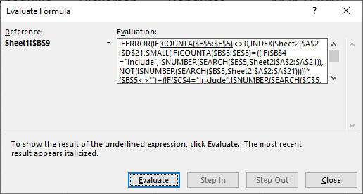
I recommend the "Evaluate Formula" tool if you are curious about a formula you don't understand. It is also great for troubleshooting formulas that return errors.
- Go to tab "Formulas" on the ribbon.
- Press with left mouse button on "Evaluate Formula" button on the ribbon. A dialog box appears, see image above.
- Press with left mouse button on "Evaluate" button to see the next calculation step.
The underlined expression shows what part of the formula that will be evaluated next. The italicized is the most recent result.
Keep press with left mouse button oning the "Evaluate button to go through all calculation steps, press with left mouse button on the "Close" button to dismiss the dialog box.
Step 1 - Search for a text string
The SEARCH function returns a number representing the position of character at which a specific text string is found reading left to right.
SEARCH(find_text,within_text, [start_num])
SEARCH($B$5, Sheet2!$A$2:$A$21)
returns {1; 1; ... ; 1}
Step 2 - Check if it is a number
The ISNUMBER function checks if a value is a number, returns TRUE or FALSE.
ISNUMBER(value)
ISNUMBER(SEARCH($B$5, Sheet2!$A$2:$A$21))
returns {TRUE; TRUE; ... ; TRUE}
Step 3 - Check if cell B4 is "Include" or Exclude"
The IF function returns one value if the logical test is TRUE and another value if the logical test is FALSE.
IF(logical_test, [value_if_true], [value_if_false])
The following part checks if cell B4 equals "Include".
IF($B$4="Include", ISNUMBER(SEARCH($B$5, Sheet2!$A$2:$A$21)), NOT(ISNUMBER(SEARCH($B$5, Sheet2!$A$2:$A$21))))
returns {FALSE; FALSE; ... ; FALSE}
Step 4 - Add all arrays
There are four similar parts in the formula described in step 1 to 3, what is different are the cell references. Each part is customized for a column, the list has four columns and the formulas has as many parts as there are columns.
The plus sign applies OR logic to the arrays, for example, 0 + 1 + 0 returns 1. If you multiply the arrays you apply AND logic. 0*1*0 equals 0.
((IF($B$4="Include", ISNUMBER(SEARCH($B$5, Sheet2!$A$2:$A$21)), NOT(ISNUMBER(SEARCH($B$5, Sheet2!$A$2:$A$21)))))*($B$5<>"")+(IF($C$4="Include", ISNUMBER(SEARCH($C$5, Sheet2!$B$2:$B$21)), NOT(ISNUMBER(SEARCH($C$5, Sheet2!$B$2:$B$21)))))*($C$5<>"")+(IF($D$4="Include", ISNUMBER(SEARCH($D$5, Sheet2!$C$2:$C$21)), NOT(ISNUMBER(SEARCH($D$5, Sheet2!$C$2:$C$21)))))*($D$5<>"")+(IF($E$4="Include", ISNUMBER(SEARCH($E$5, Sheet2!$D$2:$D$21)), NOT(ISNUMBER(SEARCH($E$5, Sheet2!$D$2:$D$21)))))*($E$5<>""))
returns {1; 1; ... ; 1}.
Step 5 - Check if the number of criteria matches the array, if it does return the corresponding row number
The COUNTA function counts the non-empty or blank cells in a cell reference.
COUNTA(value1, [value2], ...)
IF(COUNTA($B$5:$E$5)=((IF($B$4="Include", ISNUMBER(SEARCH($B$5, Sheet2!$A$2:$A$21)), NOT(ISNUMBER(SEARCH($B$5, Sheet2!$A$2:$A$21)))))*($B$5<>"")+(IF($C$4="Include", ISNUMBER(SEARCH($C$5, Sheet2!$B$2:$B$21)), NOT(ISNUMBER(SEARCH($C$5, Sheet2!$B$2:$B$21)))))*($C$5<>"")+(IF($D$4="Include", ISNUMBER(SEARCH($D$5, Sheet2!$C$2:$C$21)), NOT(ISNUMBER(SEARCH($D$5, Sheet2!$C$2:$C$21)))))*($D$5<>"")+(IF($E$4="Include", ISNUMBER(SEARCH($E$5, Sheet2!$D$2:$D$21)), NOT(ISNUMBER(SEARCH($E$5, Sheet2!$D$2:$D$21)))))*($E$5<>"")), MATCH(ROW(Sheet2!$D$2:$D$21), ROW(Sheet2!$D$2:$D$21)), "")
returns {""; ""; ""; ""; ""; ""; 7; ""; ""; ""; 11; ""; ""; ""; ""; ""; ""; 18; ""; ""}.
Now we know which records that match the conditions.
Step 6 - Find k-th smallest row number
The SMALL function returns the k-th smallest number in the array, it will also ignore text and blanks.
SMALL(IF(COUNTA($B$5:$E$5)=((IF($B$4="Include", ISNUMBER(SEARCH($B$5, Sheet2!$A$2:$A$21)), NOT(ISNUMBER(SEARCH($B$5, Sheet2!$A$2:$A$21)))))*($B$5<>"")+(IF($C$4="Include", ISNUMBER(SEARCH($C$5, Sheet2!$B$2:$B$21)), NOT(ISNUMBER(SEARCH($C$5, Sheet2!$B$2:$B$21)))))*($C$5<>"")+(IF($D$4="Include", ISNUMBER(SEARCH($D$5, Sheet2!$C$2:$C$21)), NOT(ISNUMBER(SEARCH($D$5, Sheet2!$C$2:$C$21)))))*($D$5<>"")+(IF($E$4="Include", ISNUMBER(SEARCH($E$5, Sheet2!$D$2:$D$21)), NOT(ISNUMBER(SEARCH($E$5, Sheet2!$D$2:$D$21)))))*($E$5<>"")), MATCH(ROW(Sheet2!$D$2:$D$21), ROW(Sheet2!$D$2:$D$21)), ""), ROW(A1))
becomes
SMALL({""; ""; ""; ""; ""; ""; 7; ""; ""; ""; 11; ""; ""; ""; ""; ""; ""; 18; ""; ""}, ROW(A1))
The ROW function returns the row number from the cell reference A1. A1 is a relative cell reference meaning it will change automatically when you copy the cell and paste it to adjacent cells.
and returns 7.
Step 7 - Return value from table
The INDEX function returns a value from a cell range based on a row and column number.
INDEX(Sheet2!$A$2:$D$21, SMALL(IF(COUNTA($B$5:$E$5)=((IF($B$4="Include", ISNUMBER(SEARCH($B$5, Sheet2!$A$2:$A$21)), NOT(ISNUMBER(SEARCH($B$5, Sheet2!$A$2:$A$21)))))*($B$5<>"")+(IF($C$4="Include", ISNUMBER(SEARCH($C$5, Sheet2!$B$2:$B$21)), NOT(ISNUMBER(SEARCH($C$5, Sheet2!$B$2:$B$21)))))*($C$5<>"")+(IF($D$4="Include", ISNUMBER(SEARCH($D$5, Sheet2!$C$2:$C$21)), NOT(ISNUMBER(SEARCH($D$5, Sheet2!$C$2:$C$21)))))*($D$5<>"")+(IF($E$4="Include", ISNUMBER(SEARCH($E$5, Sheet2!$D$2:$D$21)), NOT(ISNUMBER(SEARCH($E$5, Sheet2!$D$2:$D$21)))))*($E$5<>"")), MATCH(ROW(Sheet2!$D$2:$D$21), ROW(Sheet2!$D$2:$D$21)), ""), ROW(A1)), COLUMN(A1))
becomes
INDEX(Sheet2!$A$2:$D$21, 7, COLUMN(A1))
The COLUMN function returns the column number from the cell reference A1. A1 is a relative cell reference meaning it will change automatically when you copy the cell and paste it to adjacent cells.
becomes
INDEX(Sheet2!$A$2:$D$21, 7, 1)
and returns "Bronson" in cell B9.
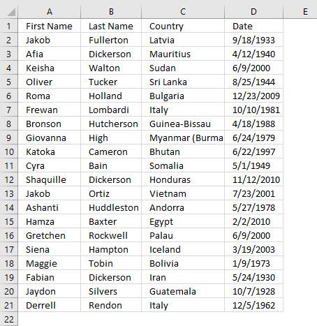
The image above shows the data source on worksheet sheet2. Bronson is found on relative row 7 in cell range Sheet2!$A$2:$D$21.
3. Wildcard lookups and include or exclude criteria - autofilter
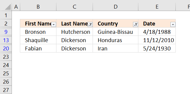
The Filter tool built-in to Excel is mostly used to filter a list based on conditions. The difference between the Filter tool and the formulas is that there are a few more extra steps to apply conditions.
The formulas are perhaps harder to enter and customize, however, once they are there they are extremely easy to use.
I will in this tutorial describe how to filter a list based on if a cell contains a specific text string and another column does not equal a specific value. Here are the steps to apply a filter using the Filter tool.
- Press with left mouse button on any cell in your data with the left mouse button.
- Go to tab "Data" on the ribbon.
- Press with left mouse button on the "Filter" button. Black arrows appear next to each column header name.
- Press with left mouse button on an arrow next to a column you want to filter.
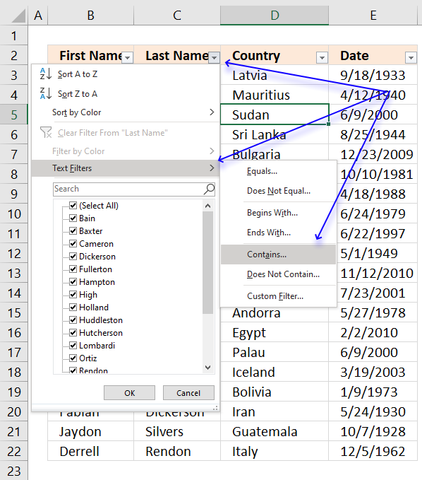
- Press with left mouse button on "Text Filters".
- Press with left mouse button on "Contains...". A dialog box appears.

- Type "son", see image above. This will filter the list if values in column name "Last name" contains "son".
- Press with left mouse button on OK button.
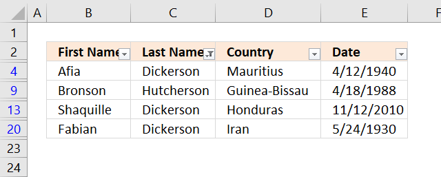
The image above shows the list after applying the first condition. Now on to the next condition.
- Press with left mouse button on the arrow next to the column name "Country".
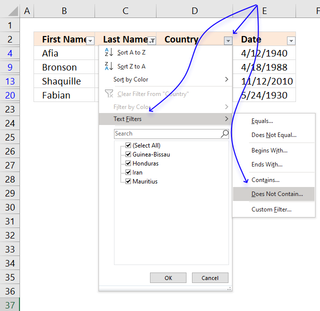
- Press with left mouse button on "Text Filters", see image above.
- Press with left mouse button on "Does Not Contain...". A dialog box appears.

- Type "Mauritius", see image above.
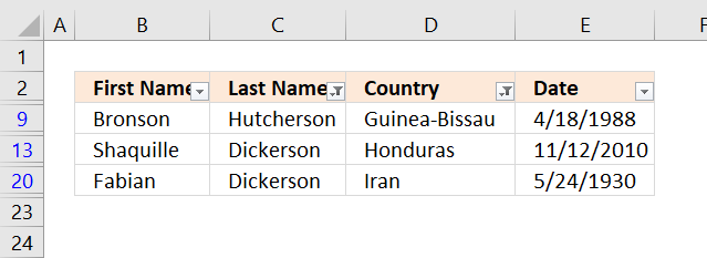
- Press with left mouse button on OK button.
Search and return multiple values category
This article demonstrates array formulas that search for cell values containing a search string and returns corresponding values on the […]
This article demonstrates formulas that let you perform partial matches based on multiple strings and return those strings if all […]
Excel categories
3 Responses to “Wildcard lookups and include or exclude criteria”
Leave a Reply
How to comment
How to add a formula to your comment
<code>Insert your formula here.</code>
Convert less than and larger than signs
Use html character entities instead of less than and larger than signs.
< becomes < and > becomes >
How to add VBA code to your comment
[vb 1="vbnet" language=","]
Put your VBA code here.
[/vb]
How to add a picture to your comment:
Upload picture to postimage.org or imgur
Paste image link to your comment.
Oh wow! Oscar you are amazing! That's absolutely brilliant and I can't wait to get into working through it and applying in my files to fully understand the details. That makes it so versatile now for me to utilise. I really don't know how to say thank you well enough. You're an absolute star and guru, thank you so much! There's beer (or whatever else you fancy) waiting for you in Oz one day! Such a fast response too, your website is an awesome resource Oscar, I've learnt so much!
Hi Oscar, I've had great progress assigning this solution for my file but I do have one more question if I may....how woudl you modify one of the Include/Exclude arrays to search for a BLANK cell. In particular I'm looking at a column of dates and want to make those with NO DATE an included search criteria. Cheers!
Dave,
Sorry, I don´t know. The COUNTA function counts values in range B5:E5. A blank is not counted.