How to use the Subtotal tool

What is the Subtotal tool?

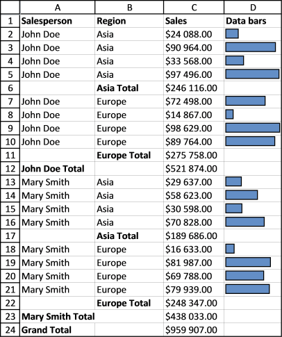
The Subtotal tool lets you insert totals and grand totals automatically. This feature was added to Excel 2010 and is still around in later Excel versions. The image above demonstrates the Subtotal tool applied to cell range B2:E30.

1. Introduction

What are the + (plus) and - (minus) signs next to row numbers?

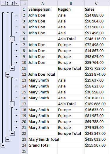
The + and minus signs to the left of the row numbers let you expand and collapse rows respectively. This functionality lets you easily examine the values behind a specific subtotal that may interest you more than the others.

What is the difference between the SUBTOTAL function and the Subtotal feature in Excel?

The SUBTOTAL function allows for various aggregate calculations (like SUM, AVERAGE) on a range with options to include or exclude hidden rows.

The Subtotal feature, on the other hand, automatically inserts SUBTOTAL functions into a dataset, organizing data into groups and providing subtotals for each group. It adds plus and minus next to row numbers which allow you to expand/collapse rows and makes it easier to examine data further.

Can I use multiple functions simultaneously with the Subtotal feature?

Yes, you can apply multiple functions by running the Subtotal feature multiple times. When adding a new subtotal make sure that the "Replace current subtotals" option is unchecked to keep existing subtotals.

How does the SUBTOTAL function handle hidden and filtered rows?

The SUBTOTAL function can include or exclude hidden rows based on the function number used. Function numbers 1-11 include hidden rows, while 101-111 exclude them. Filtered-out rows are always excluded from the calculation.

Can I create nested subtotals for more detailed data analysis?

Yes, you can create nested subtotals. First sort your data by multiple levels and then apply the Subtotal feature for each level starting from the outermost group. Make sure that you uncheck the "Replace current subtotals" option when adding additional levels.

How do I remove subtotals from my worksheet?

To remove all subtotals:

1. Go to the Data tab.
2. Press with mouse on Subtotal in the Outline group.
3. Press with left mouse button on the "Remove All" button in the Subtotal dialog box.

Can the Subtotal tool do more than totals?

Yes, it inserts the subtotal function which you can modify as you like. The subtotal function allow you to calculate not only sums but also these operations:

• AVERAGE: Returns the arithmetic mean.
• COUNT: Counts the cells containing numbers.
• COUNTA: Counts not empty cells.
• MAX: Finds the largest number.
• MIN: Finds the smallest number.
• PRODUCT: Creates a product by multiplying the numbers.
• STDEV: Calculates the standard deviation.
• STDEVP: Calculates the standard deviation based on a population.
• SUM: Adds numbers and returns a total.
• VAR: Calculates the variance.
• VARP: Calculates the variance based on a population.

The Subtotal tool is not working for me?

You need to prepare your data set by rearranging/sorting values. This is easy to do, see the next section.

2. Prepare data

Before you can use the Subtotal tool you need to prepare your data:

• Remove blank rows.
• Sort the data based on the column or columns you want to add subtotals to.

Sorting data before using the Subtotal tool in Excel is important because Subtotals group and calculate values based on changes in a specified column. The Subtotal tool inserts subtotals whenever a value in the selected column changes. If the data is unsorted, subtotals may not be applied correctly to relevant groups. Without sorting, Excel might insert subtotals at unintended places, leading to misleading results.

Sorting first helps ensure that all related records appear together, making the subtotaled report easier to read and analyze. If the data is not sorted, multiple subtotals might be added for the same category, which can cause confusion.

3. How to sort data

Excel has a built-in tool that allows you to quickly sort a data set. Here is how:

1. Press with right mouse button on on any cell in your data set. A pop-up menu appears, see image above.
2. Press with mouse on "Sort".
3. Press with left mouse button on "Custom Sort...", a dialog box appears.
   
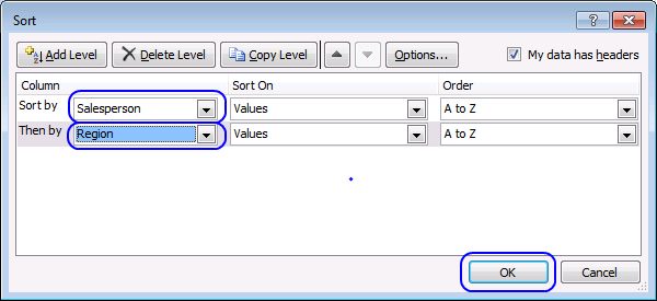
4. Sort by "Salesperson"
5. Add a Level
6. Then by "Region"
7. Press with left mouse button on OK button.

The image above shows the data set sorted based on column L and then on column M.

Back to top

Back to top

4. How to start the Subtotal tool?

The Subtotal feature is easily accessable on the ribbon, here is how:

1. Go to tab "Data" on the ribbon.
2. Press with left mouse button on the "Subtotal" button. A dialog box appears, see image above.
3. Press with left mouse button on the OK button to apply settings and create subtotals.

The image above demonstrates subtotals in cell D11 and D20 created by the Subtotal tool. The formula bar shows that the Subtotal tool inserted SUBTOTAL functions in both cell D11 and D20.

The SUBTOTAL function has many arguments which I won't be demonstrating in this article, check out the SUBTOTAL function article if you want to learn more about them.

Press with left mouse button on  symbol to collapse rows and press with left mouse button on  symbol to expand rows. You can also expand or collapse all rows on a hierarchy level by pressing 1, 2 or 3:  

These buttons are located to the left of the row numbers, see the image above or the animated image below.

Back to top

5. Subtotals on multiple levels

You can add more subtotals to your data list. We inserted subtotals before when a change occurred in column Salesperson, let's add a new subtotal for each change in column Region.

1. Select cell range A1:C20
2. Press with left mouse button on "Subtotal" button on tab "Data"
   
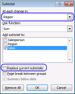
3. Press with left mouse button on the drop-down menu below the "At each change in:"
4. Select Region
5. Clear checkbox "Replace current subtotals"
6. Press with left mouse button on OK button.

6. Dialog box settings

6.1 At each change in

The first drop-down list lets you choose which column to use when determining where to insert subtotals to. When a value changes a new subtotal is inserted, this is why it is important to sort the values by salesperson first.

6.2 Use functions

The dialog box allows you to pick one function out of eleven functions, they are:

• Sum - Calculates a total.

  
  Formula in cell D11:

  =SUBTOTAL(9,D3:D10)

  Number 9 represents the SUM function, it adds numbers and returns a total.
  97496 + 33568 + 90964 + 24088 + 98629 + 72498 + 89764 + 14867 = 521874

• Count - Counts the number of cells that are not empty.

  
  Formula in cell D11:

  =SUBTOTAL(3,D3:D10)

  The first argument is 3 which represents the COUNTA function, it counts all cells that are not empty.
  There are eight cells in cell range D3:D10 and they all non-empty. The formula returns 8 in cell D11.

• Average - Returns the average (arithmetic mean) of the arguments.

  
  Formula in cell D11:

  =SUBTOTAL(1,D3:D10)

  The first argument is 1, it represents the AVERAGE function. It adds all numbers and then divides by the total count of values.
  97496 + 33568 + 90964 + 24088 + 98629 + 72498 + 89764 + 14867 = 521874
  521874/8 = 65234.25

• Max - Returns the largest number

  
  Formula in cell D11:

  =SUBTOTAL(4, D3:D10)

  Cell range D3:D10 contains the following values: 97496, 33568, 90964, 24088, 98629, 72498, 89764 and 14867.
  98629 is the largest one.

• Min - Returns the smallest number

  
  Formula in cell D11:

  =SUBTOTAL(5, D3:D10)

  Cell range D3:D10 contains the following values: 97496, 33568, 90964, 24088, 98629, 72498, 89764 and 14867.
  14867 is the smallest number.

• Product - Multiplies numbers in cell range

  
  Formula in cell D11:

  =SUBTOTAL(6, D3:D10)

  Cell range D3:D10 contains the following values: 97496, 33568, 90964, 24088, 98629, 72498, 89764 and 14867.
  97496 * 33568 * 90964 * 24088 * 98629 * 72498 * 89764 * 14867 = 6.8428772708558E+37

• Count numbers - Count the number of cells that contain numbers

  
  Formula in cell D11:

  =SUBTOTAL(2, D3:D10)

  There are eight cells in cell range D3:D10 and they all are numbers. The formula returns 8 in cell D11.

• StdDev- Calculates the standard deviation based on a sample of the entire population.

  

  Formula in cell D11:

  =SUBTOTAL(7, D3:D10)

  The first argument is 7 which represents the STDEV.S function, it was added to Excel 2010. The STDEV.S function returns the standard deviation based on a sample of the entire population.

  The standard deviation shows how much the values differ from the mean value of the group, in other words, how they are distributed around the average value, or how spread out the numbers are.

  

  x ̅ is the average.
  n is how many values.

  97496+33568+90964+24088+98629+72498+89764+14867 = 521874
  521874/8 = 65234.25 is the average number.

  (97496-65234.25)^2 + (33568-65234.25)^2 + (90964-65234.25)^2 + (24088-65234.25)^2 + (98629-65234.25)^2 + (72498-65234.25)^2 + (89764-65234.25)^2 + (14867-65234.25)^2

  becomes

  32261.75^2 + (-31666.25)^2 + 25729.75^2 + (-41146.25)^2 + 33394.75^2 + 7263.75^2 + 24529.75^2 + (-50367.25)^2

  becomes

  1040820513.0625 + 1002751389.0625 + 662020035.0625 + 1693013889.0625 + 1115209327.5625 + 52762064.0625 + 601708635.0625 +2536859872.5625

  equals 8705145725.5.

  8705145725.5/(8-1) = 1243592246.5

  1243592246.5^(1/2) = 35264.6033084168

• StdDevp - calculates the standard deviation based on the entire population

  
  Formula in cell D11:

  =SUBTOTAL(8, D3:D10)

  The STDEV.P function returns the standard deviation based on the entire population.

  

  x ̅ is the average.
  n is how many values.

  97496+33568+90964+24088+98629+72498+89764+14867 = 521874
  521874/8 = 65234.25 is the average number.

  (97496-65234.25)^2 + (33568-65234.25)^2 + (90964-65234.25)^2 + (24088-65234.25)^2 + (98629-65234.25)^2 + (72498-65234.25)^2 + (89764-65234.25)^2 + (14867-65234.25)^2

  becomes

  32261.75^2 + (-31666.25)^2 + 25729.75^2 + (-41146.25)^2 + 33394.75^2 + 7263.75^2 + 24529.75^2 + (-50367.25)^2

  becomes

  1040820513.0625 + 1002751389.0625 + 662020035.0625 + 1693013889.0625 + 1115209327.5625 + 52762064.0625 + 601708635.0625 +2536859872.5625

  equals 8705145725.5.

  8705145725.5/8 = 1088143215.6875

  1088143215.6875^(1/2) = 32987.0158651476

• Var - estimates variance based on a sample

  
  Formula in cell D11:

  =SUBTOTAL(10, D3:D10)

  The VAR.S function returns the variance based on the entire population. Variance is the average of the squared differences from the mean.

  

  x ̅ is the average.
  n is how many values.

  97496+33568+90964+24088+98629+72498+89764+14867 = 521874
  521874/8 = 65234.25 is the average number.

  (97496-65234.25)^2 + (33568-65234.25)^2 + (90964-65234.25)^2 + (24088-65234.25)^2 + (98629-65234.25)^2 + (72498-65234.25)^2 + (89764-65234.25)^2 + (14867-65234.25)^2

  becomes

  32261.75^2 + (-31666.25)^2 + 25729.75^2 + (-41146.25)^2 + 33394.75^2 + 7263.75^2 + 24529.75^2 + (-50367.25)^2

  becomes

  1040820513.0625 + 1002751389.0625 + 662020035.0625 + 1693013889.0625 + 1115209327.5625 + 52762064.0625 + 601708635.0625 +2536859872.5625

  equals 8705145725.5.

  8705145725.5/(8-1) = 1243592246.5

• Varp - estimates variance based on population

  
  Formula in cell D11:

  =SUBTOTAL(10, D3:D10)

  The VAR.P function returns the variance based on the entire population. Variance is the average of the squared differences from the mean.

  
  x ̅ is the average.
  n is how many values.

  97496+33568+90964+24088+98629+72498+89764+14867 = 521874
  521874/8 = 65234.25 is the average number.

  (97496-65234.25)^2 + (33568-65234.25)^2 + (90964-65234.25)^2 + (24088-65234.25)^2 + (98629-65234.25)^2 + (72498-65234.25)^2 + (89764-65234.25)^2 + (14867-65234.25)^2

  becomes

  32261.75^2 + (-31666.25)^2 + 25729.75^2 + (-41146.25)^2 + 33394.75^2 + 7263.75^2 + 24529.75^2 + (-50367.25)^2

  becomes

  1040820513.0625 + 1002751389.0625 + 662020035.0625 + 1693013889.0625 + 1115209327.5625 + 52762064.0625 + 601708635.0625 +2536859872.5625

  equals 8705145725.5.

  8705145725.5/8 = 1088143215.6875

6.3 Add subtotal to

This setting allows you to choose which columns to add subtotals to.

6.4 Replace current subtotals

This checkbox lets you substitute current subtotals with new ones, if enabled.

6.5 Pagebreak between groups

This checkbox, if enabled, lets you put each group in a new page.

6.6 Summary below data

The last checkbox adds a summary below all groups, for example, if a total is calculated for each group then a grand total is calculated below all groups.

6.7 Add data bars

Now it is time to spice up your data table with some chart bars. Hold on, I am not going to insert a chart. Conditional Formatting is what we are going to use actually.

1. Create a new column and type =C2 in cell D2.
2. Copy cell D2 to the cells below.
3. Remove cells that link to subtotals and grand total.
4. Select cell range D2:D24.
5. Go to tab "Home" on the ribbon.
6. Press with left mouse button on "Conditional formatting" button.
7. Press with left mouse button on "Data Bars".
8. Press with left mouse button on "More Rules..."
   
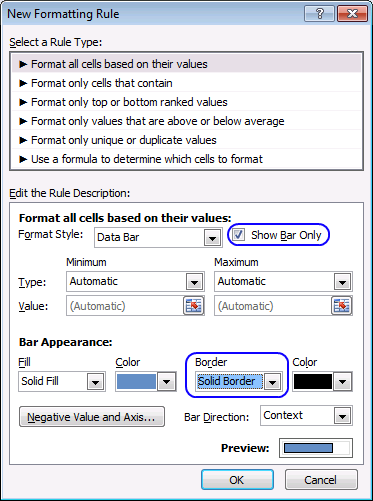
9. Enable the checkbox "Show Bar Only".
10. I chose a "Solid Border" from the "Border" drop-down menu.
11. Press with left mouse button on OK button.

The Data Bars let you quickly compare numbers, finding outliers, or interesting statistics.

7. Remove all subtotals

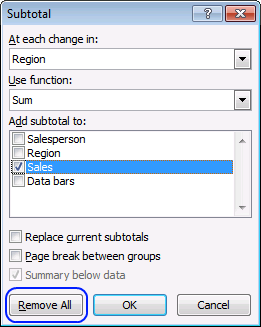
You can easily remove all subtotals, select the cell range you want to remove subtotals from. Go to tab "Data", press with left mouse button on "Subtotal" button. Press with left mouse button on "Remove All" button.

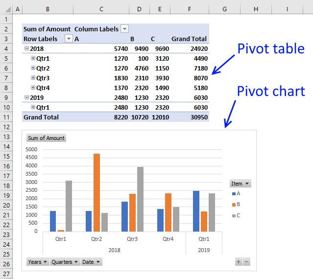
Tip! Build a Pivot Table/Pivot chart

A pivot table allows you to summarize a data table in many different ways, using different criteria. It is easy and you will be analyzing your data in no time. Pivot tables are subtotals on steroids.

I highly recommend reading this blog post: Analyze trends using pivot tables, there is also a quick introduction to pivot tables.

You can also compare data, year to year, month to month and whatever time frame you like.

Features category

More than 1300 Excel formulas

Excel categories

Leave a Comment