How to use the TRIMMEAN function

What is the TRIMMEAN function?

The TRIMMEAN function calculates the mean of the interior of a data set. The function excludes a percentage of data points from the top and bottom tails of a data set, use it to exclude outlying data from your analysis.

1. Introduction

What is trim?

Trim refers to excluding specific values from a group of values, in this case the top and bottom values.

What is the mean?

The arithmetic mean is calculated by dividing the sum of all values by the number of values.

For example, an array contains these values: 3,2,1

The sum is 3 + 2 + 1 equals 6
The number of values is 3.
6/3 equals 2. The average of 3, 2, 1 is 2

What is the interior of a data set?

In statistics and data analysis, the interior and tails refer to different regions within the distribution of a data set:

Interior - The interior of a data set refers to the main body or central region, excluding the outer extremities. It contains the bulk of the values clustered around the center of the distribution (e.g. near the median).

What are the bottom and top tails of a data set?

Bottom/Left Tail - The bottom or left tail encompasses the lowest, smallest values that extend leftwards from the main body. This includes extreme low outliers.

Top/Right Tail - The top or right tail encompasses the highest, largest values that extend rightwards from the main body. This includes extreme high outliers.

Does the TRIMMEAN function exclude the same number of data points from top and bottom?

The TRIMMEAN function rounds the number of excluded data points to the nearest multiple of 2 to create symmetry and exclude the same number of data points from top and bottom.

Example, if there are 100 data points and the percentage is 0.01 then 2 values are excluded even though 0.01 * 100 = 1.

What is the nearest multiple of 2?

The nearest multiple of 2 to a number refers to the closest integer that is divisible by 2.

Some examples of nearest multiple of 2 to

• 5 is 6
• 19 is 20
• 14 is 14

2. TRIMMEAN Function Syntax

TRIMMEAN(array, percent)

3. TRIMMEAN Function Arguments

array	Required. The values to trim and average.
percent	Required. The fractional number of data points to exclude from the calculation. If percent is 0.2 and there are 100 data points, 20 data points are excluded.

What is a fractional number?

A fractional number represents a part or portion of a whole number. It expresses a ratio of two integers and consists of a numerator and denominator separated by a fraction bar. For example: 1/8, 6/19, 2/39.

4. TRIMMEAN Function Example 1

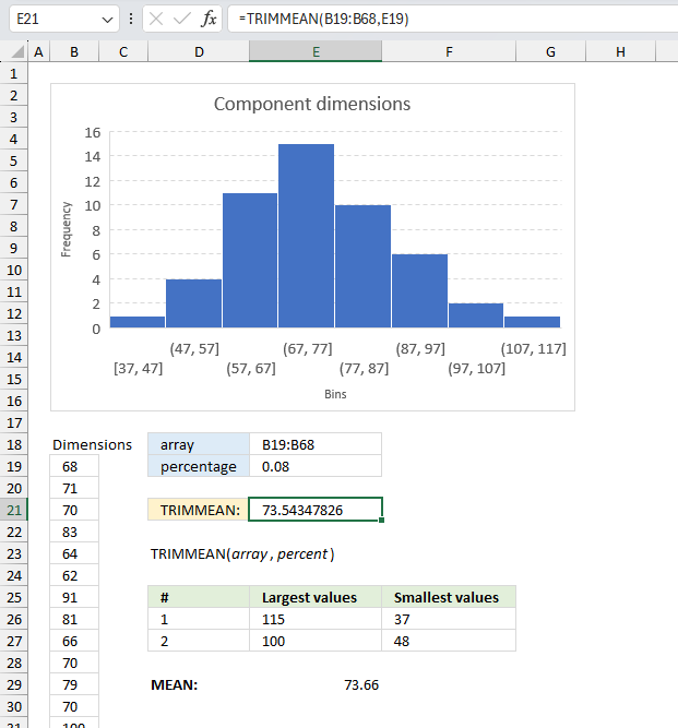
A manufacturing process produces a batch of components, and quality control measures the dimensions of each component. To assess the overall quality, the engineer wants to calculate the mean dimension while excluding the top 4% and bottom 4% of measurements, which may be due to measurement errors or defective components. How can the TRIMMEAN function help in this situation?

The data is displayed in cell range B19:B68, here are the data points:

68	79	80	70	80
71	70	95	89	48
70	100	80	51	84
83	59	76	59	52
64	115	65	65	76
62	86	50	58	71
91	87	77	81	70
81	64	37	63	99
66	91	76	63	71
70	72	88	68	92

The arguments are:

• array = B19:B68
• percentage = 0.08 (8%)

The data contains 50 individual data points. 8% of 50 equals 4. This means that the two largest and two smallest data points are excluded from the calculation.

The two smallest data points are: 37 and 48. The two largest data points are 115 and 100. These four combined values are excluded.

Formula in cell E21:

The result in cell E21 is 73.54. Lets see if this number is correct. If we exclude values 37, 48, 100, and 115 we get a mean of 73.54

68+71+70+83+64+62+91+81+66+70+79+70+0+59+0+86+87+64+91+72+80+95+80+76+65+50+77+76+88+70+89+51+59+65+58+81+63+63+68+80+84+52+76+71+70+99+71+92 equals 3383

3383 / 46 equals 73.54 The calculation is correct.

The displayed visual representation is a histogram, which illustrates the distribution of the data by categorizing it into distinct value ranges known as bins. Each bin represents a specific interval within which data points may fall. The vertical axis, or the y-axis, depicts the frequency or count of data points that belong to each corresponding bin. In other words, the height of each bar on the histogram indicates the number of observations or occurrences that lie within the specified bin's range.

Number 37 is in the leftmost bin, 48 is in the second bin from the left. Number 100 is in the 7th bin and the largest value of them all 115 is in the last (8th) bin.

Cells E26:E27 calculate the largest and second largest value and cells F26:F27 calculate the smallest and next smallest value, from cell range B19:B68.

5. TRIMMEAN Function Example 2

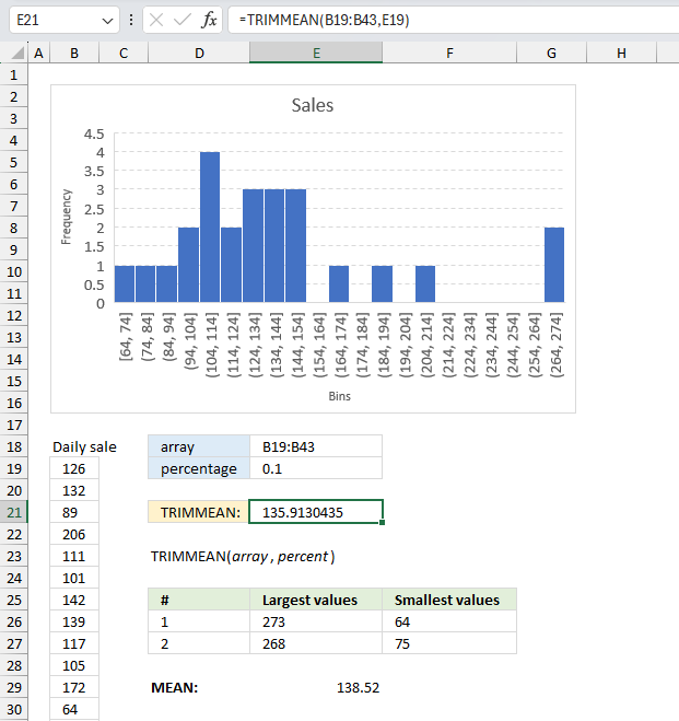
A company tracks the daily sales of its products. To get a more representative average, the sales manager wants to calculate the mean daily sales while excluding the top 5% and bottom 5% sales figures, which may be influenced by unusual events. How can the TRIMMEAN function help in this scenario?

The data is shown in cell range B19:B43, here are the data points:

126	101	172	268	139
132	142	64	101	128
89	139	121	75	146
206	117	273	190	107
111	105	112	153	146

The arguments are:

• array = B19:B43
• percentage = 0.1 (10%)

The data contains 50 individual data points. 10% of 25 equals 2.4. The nearest multiple of 2.4 is 2. This means that the largest and smallest data points are excluded from the calculation.

The smallest data points is 64 and the largest data points is 273, these two combined values are excluded.

Formula in cell E21:

The result in cell E21 is 135.91. Lets see if this number is correct. If we exclude values 37, 48, 100, and 115 we get a mean of 135.91

126+132+89+206+111+101+142+139+117+105+172+121+112+268+101+75+190+153+139+128+146+107+146 equals 3126

3126 / 23 equals 135.91. The calculation is correct.

The image above shows a histogram which displays the distribution of the data grouped into bins. A bin is an interval that data points may fall into. The y axis shows the frequency of each bin meaning how many data points that fall into each specified bin.

Cell E26 calculates the largest value and cell F26 calculates the smallest value, from cell range B19:B43.

6. How is the TRIMMEAN Function calculated?

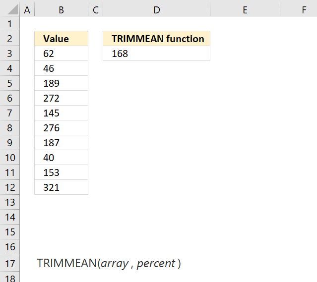
Formula in cell D3:

The values are: 62, 46, 189, 272, 145, 276, 187, 40, 153, and 321 and the count is 10.

40% of 10 is 4, the two largest and the two smallest values are excluded. The two top values are: 321 and 276 and the bottom values are 40 and 46.

The average of the remaining values is 62 + 189 + 272 + 145 + 187 + 153 = 1008 , 1008 / 6 equals 168

7. Function not working

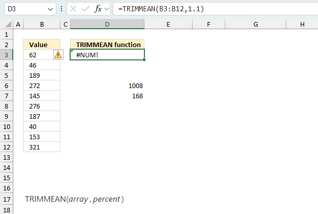
TRIMMEAN returns the #NUM! error value if the percent argument is less than 0 (zero) or larger than 1.

7.1 Troubleshooting the error value

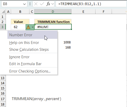
When you encounter an error value in a cell a warning symbol appears, displayed in the image above. Press with mouse on it to see a pop-up menu that lets you get more information about the error.

1. The first line describes the error if you press with left mouse button on it.
2. The second line opens a pane that explains the error in greater detail.
3. The third line takes you to the "Evaluate Formula" tool, a dialog box appears allowing you to examine the formula in greater detail.
4. This line lets you ignore the error value meaning the warning icon disappears, however, the error is still in the cell.
5. The fifth line lets you edit the formula in the Formula bar.
6. The sixth line opens the Excel settings so you can adjust the Error Checking Options.

Here are a few of the most common Excel errors you may encounter.

#NULL error - This error occurs most often if you by mistake use a space character in a formula where it shouldn't be. Excel interprets a space character as an intersection operator. If the ranges don't intersect an #NULL error is returned. The #NULL! error occurs when a formula attempts to calculate the intersection of two ranges that do not actually intersect. This can happen when the wrong range operator is used in the formula, or when the intersection operator (represented by a space character) is used between two ranges that do not overlap. To fix this error double check that the ranges referenced in the formula that use the intersection operator actually have cells in common.

#SPILL error - The #SPILL! error occurs only in version Excel 365 and is caused by a dynamic array being to large, meaning there are cells below and/or to the right that are not empty. This prevents the dynamic array formula expanding into new empty cells.

#DIV/0 error - This error happens if you try to divide a number by 0 (zero) or a value that equates to zero which is not possible mathematically.

#VALUE error - The #VALUE error occurs when a formula has a value that is of the wrong data type. Such as text where a number is expected or when dates are evaluated as text.

#REF error - The #REF error happens when a cell reference is invalid. This can happen if a cell is deleted that is referenced by a formula.

#NAME error - The #NAME error happens if you misspelled a function or a named range.

#NUM error - The #NUM error shows up when you try to use invalid numeric values in formulas, like square root of a negative number.

#N/A error - The #N/A error happens when a value is not available for a formula or found in a given cell range, for example in the VLOOKUP or MATCH functions.

#GETTING_DATA error - The #GETTING_DATA error shows while external sources are loading, this can indicate a delay in fetching the data or that the external source is unavailable right now.

7.2 The formula returns an unexpected value

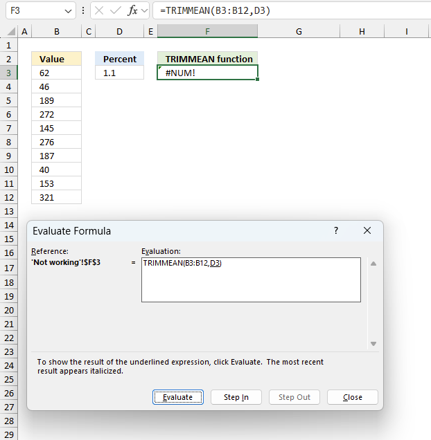
To understand why a formula returns an unexpected value we need to examine the calculations steps in detail. Luckily, Excel has a tool that is really handy in these situations. Here is how to troubleshoot a formula:

1. Select the cell containing the formula you want to examine in detail.
2. Go to tab “Formulas” on the ribbon.
3. Press with left mouse button on "Evaluate Formula" button. A dialog box appears.
   The formula appears in a white field inside the dialog box. Underlined expressions are calculations being processed in the next step. The italicized expression is the most recent result. The buttons at the bottom of the dialog box allows you to evaluate the formula in smaller calculations which you control.
4. Press with left mouse button on the "Evaluate" button located at the bottom of the dialog box to process the underlined expression.
5. Repeat pressing the "Evaluate" button until you have seen all calculations step by step. This allows you to examine the formula in greater detail and hopefully find the culprit.
6. Press "Close" button to dismiss the dialog box.

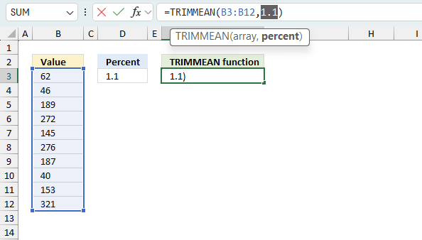
There is also another way to debug formulas using the function key F9. F9 is especially useful if you have a feeling that a specific part of the formula is the issue, this makes it faster than the "Evaluate Formula" tool since you don't need to go through all calculations to find the issue..

1. Enter Edit mode: Double-press with left mouse button on the cell or press F2 to enter Edit mode for the formula.
2. Select part of the formula: Highlight the specific part of the formula you want to evaluate. You can select and evaluate any part of the formula that could work as a standalone formula.
3. Press F9: This will calculate and display the result of just that selected portion.
4. Evaluate step-by-step: You can select and evaluate different parts of the formula to see intermediate results.
5. Check for errors: This allows you to pinpoint which part of a complex formula may be causing an error.

The image above shows cell reference D3 converted to hard-coded value using the F9 key. The TRIMMEAN function requires numerical values between 0 (zero) and 1 which is not the case in this example. We have found what is wrong with the formula.

Tips!

• View actual values: Selecting a cell reference and pressing F9 will show the actual values in those cells.
• Exit safely: Press Esc to exit Edit mode without changing the formula. Don't press Enter, as that would replace the formula part with the calculated value.
• Full recalculation: Pressing F9 outside of Edit mode will recalculate all formulas in the workbook.

Remember to be careful not to accidentally overwrite parts of your formula when using F9. Always exit with Esc rather than Enter to preserve the original formula. However, if you make a mistake overwriting the formula it is not the end of the world. You can “undo” the action by pressing keyboard shortcut keys CTRL + z or pressing the “Undo” button

7.3 Other errors

Floating-point arithmetic may give inaccurate results in Excel - Article

Floating-point errors are usually very small, often beyond the 15th decimal place, and in most cases don't affect calculations significantly.

Functions in 'Statistical' category

The TRIMMEAN function function is one of 73 functions in the 'Statistical' category.

Excel function categories

Excel categories

Leave a Comment