How to use the SHEETS function

What is the SHEETS function?

The SHEETS function returns the number of sheets in a cell reference. It returns the total number of sheets in a workbook if the argument is omitted.

1. Introduction

What is a cell reference?

A cell reference lets you "fetch" and use values in other cells in a formula.

There are two styles of cell references:

• A1-style reference. The A1-style reference is the default style in Excel, it names columns by letters from A to Z. After Z it starts over with AA, AB, and so on until XFD. Rows are numbered from 1 to 1048576, older Excel versions use less row numbers.
• R1C1-style reference. The R1C1-style uses row number and column number like: R1C1, R2C5 and R10C15. Rows are labeled R1, R2, R3 and so on, columns are labeled C1, C2, C3 etc.

The A1-style reference notation is the most common one, here are some examples:

• A1 - single cell reference on the same worksheet
• A1:D5 - reference to a cell range on the same worksheet
• Budget!Z3 - a single cell reference to worksheet Budget
• 'Budget 2050'!A3 - a single cell reference to a worksheet containing a space character

There are two types of cell references:

• Relative cell references
• Absolute cell references

The examples above are all relative cell references, they change accordingly if a cell is copied and pasted to another cell which absolute cell references do not. The $ dollar character lets you an absolute cell reference meaning you can lock a cell reference horizontally, vertically or both. Here are a few examples:

• A1 is a relative cell reference. It will change when the cell is copied to another cell.
• A$1 has a relative column reference but an absolute row reference, this means that the column letter may change if the cell is copied and pasted to cells in another column than A.
• $A$1 has absolute cell references for both the row and column parts. Nothing changes in the cell reference when you copy the cell and paste it to another cell.

What is a worksheet?

A worksheet is a single page in an Excel workbook sometimes also called only sheet. You can see the different worksheets in your open workbook by examining the tabs located in the bottom of the worksheet. The tabs have names that you can rename but they also have a sheet number that represents the order or rank in the workbook. The first tab which is the bottom most left one is numbered 1, the next one is the second worksheet and so on.

The worksheet contains a cell grid where you can enter, organize, manipulate and analyze data. Excel allows worksheets within a workbook to have different visibility states:

• Visible worksheet: Worksheet is fully visible and interactive in the workbook, the tab is shown at the bottom. This state is default for new worksheets.
• Hidden worksheet: Not visible but can be made visible using the Unhide command, the tab is hidden at the bottom of the worksheet which makes it impossible to select it. This state is useful for hiding data but keeping it accessible.
• Very hidden worksheet: Not visible and not accessible via the Unhide command, the tab is hidden at the bottom. A worksheet can only be made "very hidden" using VBA or the Visual Basic Editor.

Does the SHEETS function work with 3d-ranges?

Yes, the SHEETS function work with 3d-ranges, see the example below in section 3.

2. Syntax

SHEETS(reference)

reference

Optional. The reference you want to determine the number of sheets it contains.

3. Example 1

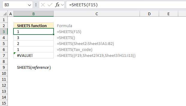
This image shows examples of the SHEETS function in Excel and its various use cases. Column A (B2:B7) shows the results of different SHEETS function calls. Column B (C2:C7) shows the corresponding formulas used. The SHEETS function is used to count the number of sheets in a workbook or a specified reference.

The following formula counts the number of worksheets in cell reference F15.

Formula in cell D3:

This formula returns 1 which represents the number of sheets in cell reference F15. This reference points to cell F15 on the same worksheet since the worksheet name is omitted from the cell reference.

Formula in cell D4:

This formula returns 3 meaning there are three worksheets in this workbook. If no argument is specified the SHEETS function returns the total number of sheets in this workbook.

Formula in cell D5:

This formula returns 2 which represents the number of sheets in cell reference Sheet2:Sheet3!A1:B2. This reference is a 3d-reference that points to multiple worksheets.

Formula in cell D6:

This formula returns 1 which represents the number of sheets in the named range Tax_code. This named range points to Sheet2!$G$13 which is cell G13 on worksheet Sheet2.

Formula in cell D6:

This formula returns an #VALUE! error which confirms that the SHEETS function can't handle multiple cell references.

4. Example 2

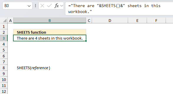
This example shows how to display the count of worksheets in the current workbook. Cell B3 contains a formula that combines text and the total count of worksheets.

Formula in cell B3:

This formula combines text with the SHEETS() function to create a dynamic sentence that reports the number of sheets in the current workbook.

• SHEETS(): This function, when used without arguments, returns the total number of sheets in the active workbook.
• "&": The ampersands are used for string concatenation in Excel, joining text and the result of the SHEETS() function.
• "There are " and " sheets in this workbook.": These are text strings that form the beginning and end of the sentence.

When Excel evaluates this formula, it:

1. Calculates the result of SHEETS() which in this case is 4.
2. Concatenates this number with the surrounding text.

The result, as shown in cell B3, is: "There are 4 sheets in this workbook.". This formula is useful for automatically updating the sheet count whenever sheets are added or removed from the workbook. This formula provides a dynamic way to display this information.

5. Function not working

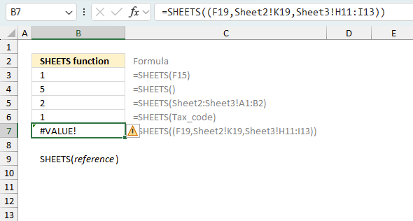
The SHEETS function returns

• #REF! error value if reference is not a valid value.
• #VALUE! error if the an invalid number of references are used.
• #NAME? error if you misspell the function name.

5.1 Troubleshooting the error value

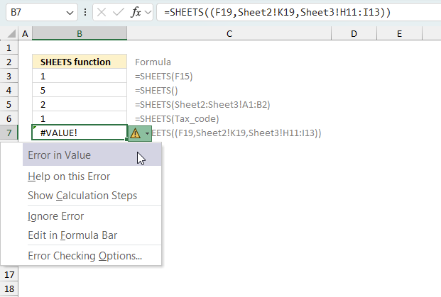
When you encounter an error value in a cell a warning symbol appears, displayed in the image above. Press with mouse on it to see a pop-up menu that lets you get more information about the error.

1. The first line describes the error if you press with left mouse button on it.
2. The second line opens a pane that explains the error in greater detail.
3. The third line takes you to the "Evaluate Formula" tool, a dialog box appears allowing you to examine the formula in greater detail.
4. This line lets you ignore the error value meaning the warning icon disappears, however, the error is still in the cell.
5. The fifth line lets you edit the formula in the Formula bar.
6. The sixth line opens the Excel settings so you can adjust the Error Checking Options.

Here are a few of the most common Excel errors you may encounter.

#NULL error - This error occurs most often if you by mistake use a space character in a formula where it shouldn't be. Excel interprets a space character as an intersection operator. If the ranges don't intersect an #NULL error is returned. The #NULL! error occurs when a formula attempts to calculate the intersection of two ranges that do not actually intersect. This can happen when the wrong range operator is used in the formula, or when the intersection operator (represented by a space character) is used between two ranges that do not overlap. To fix this error double check that the ranges referenced in the formula that use the intersection operator actually have cells in common.

#SPILL error - The #SPILL! error occurs only in version Excel 365 and is caused by a dynamic array being to large, meaning there are cells below and/or to the right that are not empty. This prevents the dynamic array formula expanding into new empty cells.

#DIV/0 error - This error happens if you try to divide a number by 0 (zero) or a value that equates to zero which is not possible mathematically.

#VALUE error - The #VALUE error occurs when a formula has a value that is of the wrong data type. Such as text where a number is expected or when dates are evaluated as text.

#REF error - The #REF error happens when a cell reference is invalid. This can happen if a cell is deleted that is referenced by a formula.

#NAME error - The #NAME error happens if you misspelled a function or a named range.

#NUM error - The #NUM error shows up when you try to use invalid numeric values in formulas, like square root of a negative number.

#N/A error - The #N/A error happens when a value is not available for a formula or found in a given cell range, for example in the VLOOKUP or MATCH functions.

#GETTING_DATA error - The #GETTING_DATA error shows while external sources are loading, this can indicate a delay in fetching the data or that the external source is unavailable right now.

5.2 The formula returns an unexpected value

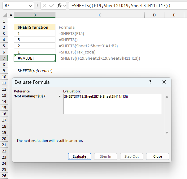
To understand why a formula returns an unexpected value we need to examine the calculations steps in detail. Luckily, Excel has a tool that is really handy in these situations. Here is how to troubleshoot a formula:

1. Select the cell containing the formula you want to examine in detail.
2. Go to tab “Formulas” on the ribbon.
3. Press with left mouse button on "Evaluate Formula" button. A dialog box appears.
   The formula appears in a white field inside the dialog box. Underlined expressions are calculations being processed in the next step. The italicized expression is the most recent result. The buttons at the bottom of the dialog box allows you to evaluate the formula in smaller calculations which you control.
4. Press with left mouse button on the "Evaluate" button located at the bottom of the dialog box to process the underlined expression.
5. Repeat pressing the "Evaluate" button until you have seen all calculations step by step. This allows you to examine the formula in greater detail and hopefully find the culprit.
6. Press "Close" button to dismiss the dialog box.

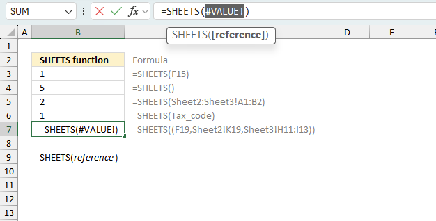
There is also another way to debug formulas using the function key F9. F9 is especially useful if you have a feeling that a specific part of the formula is the issue, this makes it faster than the "Evaluate Formula" tool since you don't need to go through all calculations to find the issue..

1. Enter Edit mode: Double-press with left mouse button on the cell or press F2 to enter Edit mode for the formula.
2. Select part of the formula: Highlight the specific part of the formula you want to evaluate. You can select and evaluate any part of the formula that could work as a standalone formula.
3. Press F9: This will calculate and display the result of just that selected portion.
4. Evaluate step-by-step: You can select and evaluate different parts of the formula to see intermediate results.
5. Check for errors: This allows you to pinpoint which part of a complex formula may be causing an error.

The image above shows cell reference (F19,Sheet2!K19,Sheet3!H11:I13) converted to hard-coded value using the F9 key. The SHEETS function requires a valid cell reference which is not the case in this example. We have found what is wrong with the formula.

Tips!

• View actual values: Selecting a cell reference and pressing F9 will show the actual values in those cells.
• Exit safely: Press Esc to exit Edit mode without changing the formula. Don't press Enter, as that would replace the formula part with the calculated value.
• Full recalculation: Pressing F9 outside of Edit mode will recalculate all formulas in the workbook.

Remember to be careful not to accidentally overwrite parts of your formula when using F9. Always exit with Esc rather than Enter to preserve the original formula. However, if you make a mistake overwriting the formula it is not the end of the world. You can “undo” the action by pressing keyboard shortcut keys CTRL + z or pressing the “Undo” button

7.3 Other errors

Floating-point arithmetic may give inaccurate results in Excel - Article

Floating-point errors are usually very small, often beyond the 15th decimal place, and in most cases don't affect calculations significantly.

Functions in 'Information' category

The SHEETS function function is one of 19 functions in the 'Information' category.

Excel function categories

Excel categories

Leave a Comment