How to use the N function

What is the N function?

The N function returns a value converted into a number.

1. Introduction

How does Excel handle value data types?

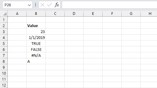
Excel changes the position of the value in a cell based on the value type. For example:

• Cells B2 and B8 contain text values that are aligned left.
• Cell B3 contains a number that is right aligned in the cell.
• Cell B4 contains a date, which Excel handles as a number. The date is right aligned.
• Cells B5 and B6 contain boolean values, which are automatically centered in the cell.
• Cell B7 contains an error value, which is also centered.

Note, the user may have changed the cell formatting making these guidelines useless. To revert back to default settings check that the align buttons are not selected:

• Align left
• Center
• Align right

What is the difference between the T and N function?

The T function deletes numbers and dates, the N function removes text values and returns 0 (zero).

What other functions let you identify/format/convert values?

ISTEXT function | TEXT function | VALUETOTEXT function | T function

2. Syntax

N(value)

value

Required. The value you want to convert.

3. Example 1

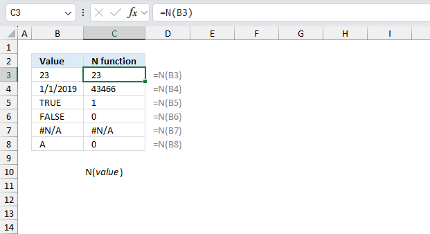
The N function in cell C3 contains a cell reference to cell B2. B2 contains a number, the N function returns the number.

Formula in cell C3:

Cell B4 contains a date, Excel dates are actually numbers and the N function returns the number itself. Excel represents dates as serial numbers, where each date is assigned a unique number starting from January 1, 1900, which is represented as the serial number 1 and 43466 represents 1/1/2019. The serial number representation of dates allows you to perform various calculations with dates in Excel. Adding or subtracting a number to a date serial number will result in a new date serial number, which can then be formatted as a date.

Cells B5 and B6 are TRUE and FALSE respectively, the N function returns the corresponding numerical values which are 1 and 0. There are other ways you can convert boolean values like adding 0 (zero) TRUE + 0 = 1 or FALSE + 0 = 0. Multiplying by 1: TRUE * 1 = 1 and FALSE * 1 = 0

Cells B7 contains an error value and the N function returns the same error value.You need a method to catch or trap errors before they are processed by the N function. You have the following options among others:

• The IFERROR function allows you to specify an alternative value to be returned if the formula encounters an error.
• The ISERROR function checks if a formula or value contains an error and returns TRUE if an error is present, and FALSE otherwise.

Cell B8 contains a text value, but the text value is ignored and 0 (zero) is returned instead.

4. Example 2

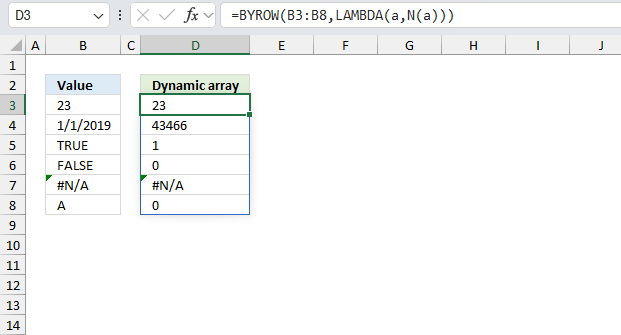
The N function can't take an array as input value, however, there is a workaround based on the new BYROW function. The image above contains random values in cell range B3:B8. Excel 365 dynamic array formula in cell D3:

The formula in cell D3 works only in Excel 365, it returns an array of values that spills to adjacent cells, in this case, to cell D3 and cells below. The BYROW function allows us to pass values, one by one, to the N function and then return a dynamic array that spills to cells below as far as needed.

The formula is a combination of three Excel functions

1. BYROW(): This function applies a specified operation to each row of a range and returns the results as an array.
2. LAMBDA(): This function allows you to define a custom function that can be used within the BYROW() function.
3. N function: Converts a value into a number.

Here's a breakdown of what this formula does:

1. B3:B8: This is the range of cells that the formula is being applied to.
2. LAMBDA(a,N(a)): This is the custom function being defined using the LAMBDA() function. The function takes two arguments:
   • a: This represents the current row being processed.
   • N(a): The N() function is used to convert the value in the current row to a numeric value.
3. BYROW(B3:B8,LAMBDA(a,N(a))): The BYROW() function applies the custom function defined by LAMBDA(a,N(a)) to each row of the range B3:B8. The result is an array of the numeric values for each row.

This technique allows us to use arrays with the N function which was not possible in earlier Excel versions.

5. Example 3

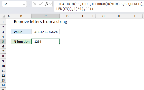
This example utilizes the N functions ability to convert text values to 0 (zeros). In other words, the formula in cell C5 extracts the numbers only from the string in cell C3. Cell C3 contains: ABC123CDG4VX

Formula in cell C5:

If we remove the letters from the string we get 1234 filtering out ABCCDGV and X. Here is how the formula works:

1. LEN(C3): Counts the number of characters in cell C3.
2. SEQUENCE(,LEN(C3)): Creates a sequence from 1 to n, n represents the number of characters in cell C3.
3. MID(C3,SEQUENCE(,LEN(C3)),1): Extract each character into one array. Each container in the array has a single character. The position in the array determines which character in the string.
4. MID(C3,SEQUENCE(,LEN(C3)),1)*1: The asterisk allows us to multiply each character by 1 which converts text values to numbers.
5. N(MID(C3,SEQUENCE(,LEN(C3)),1)*1): The N function converts text values to 0 (zero).
6. IFERROR(N(MID(C3,SEQUENCE(,LEN(C3)),1)*1),""): The IFERROR function catches errors and replaces them with nothing "".
7. TEXTJOIN("",TRUE,IFERROR(N(MID(C3,SEQUENCE(,LEN(C3)),1)*1),"")): Appends all remaining values and returns a string containing only single digits.

6. Function not working

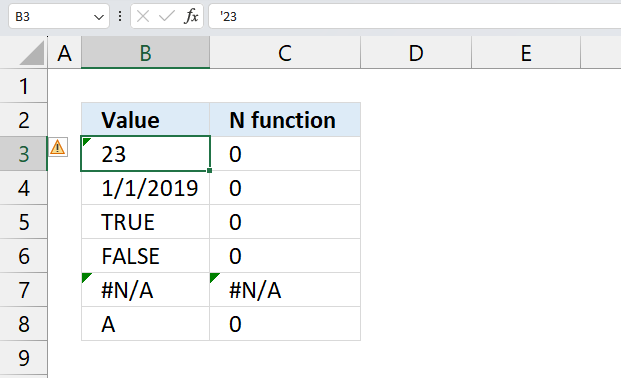
The above image shows that the N function doesn't return numbers, dates and boolean values, why does that happen? Select these cells to evaluate the values in the formula bar.

The apostrophe character converts numbers, dates and boolean values to text values, there is no way to tell unless you select one of the values and examine the formula bar. This sometimes happen when you import data from databases, the internet, and other sources.

The #NAME error appears if the function name is misspelled.

Other errors may have their origin in the source data. Check the source data for errors.

Can I use the N function in an array formula?

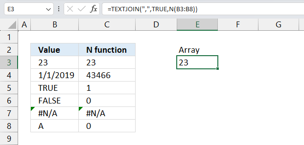
No, it returns only the first value in an array. The example above demonstrates that the N function returns the first value in the cell range B3:B8 which is 23. The remaining values in cell range B3:B8 are ignored.

However, Excel 365 subscribers can use arrays if they implement the fairly new BYROW function demonstrated in section 4 example 2 above.

6.1 Troubleshooting the error value

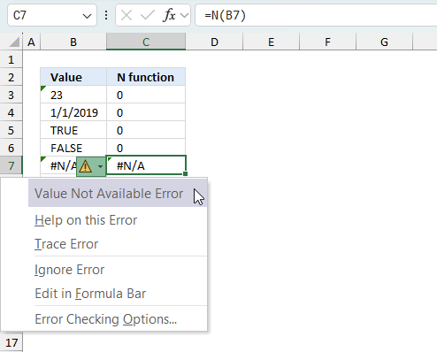
When you encounter an error value in a cell a warning symbol appears, displayed in the image above. Press with mouse on it to see a pop-up menu that lets you get more information about the error.

1. The first line describes the error if you press with left mouse button on it.
2. The second line opens a pane that explains the error in greater detail.
3. The third line takes you to the "Evaluate Formula" tool, a dialog box appears allowing you to examine the formula in greater detail.
4. This line lets you ignore the error value meaning the warning icon disappears, however, the error is still in the cell.
5. The fifth line lets you edit the formula in the Formula bar.
6. The sixth line opens the Excel settings so you can adjust the Error Checking Options.

Here are a few of the most common Excel errors you may encounter.

#NULL error - This error occurs most often if you by mistake use a space character in a formula where it shouldn't be. Excel interprets a space character as an intersection operator. If the ranges don't intersect an #NULL error is returned. The #NULL! error occurs when a formula attempts to calculate the intersection of two ranges that do not actually intersect. This can happen when the wrong range operator is used in the formula, or when the intersection operator (represented by a space character) is used between two ranges that do not overlap. To fix this error double check that the ranges referenced in the formula that use the intersection operator actually have cells in common.

#SPILL error - The #SPILL! error occurs only in version Excel 365 and is caused by a dynamic array being to large, meaning there are cells below and/or to the right that are not empty. This prevents the dynamic array formula expanding into new empty cells.

#DIV/0 error - This error happens if you try to divide a number by 0 (zero) or a value that equates to zero which is not possible mathematically.

#VALUE error - The #VALUE error occurs when a formula has a value that is of the wrong data type. Such as text where a number is expected or when dates are evaluated as text.

#REF error - The #REF error happens when a cell reference is invalid. This can happen if a cell is deleted that is referenced by a formula.

#NAME error - The #NAME error happens if you misspelled a function or a named range.

#NUM error - The #NUM error shows up when you try to use invalid numeric values in formulas, like square root of a negative number.

#N/A error - The #N/A error happens when a value is not available for a formula or found in a given cell range, for example in the VLOOKUP or MATCH functions.

#GETTING_DATA error - The #GETTING_DATA error shows while external sources are loading, this can indicate a delay in fetching the data or that the external source is unavailable right now.

6.2 The formula returns an unexpected value

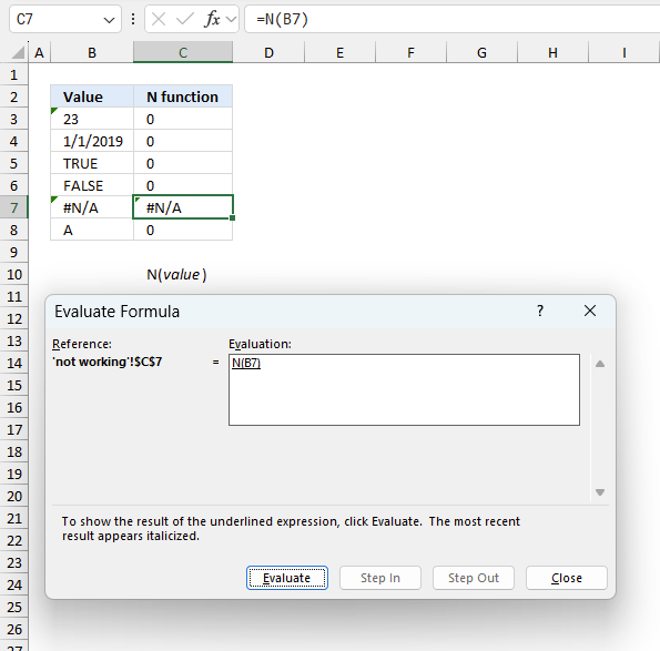
To understand why a formula returns an unexpected value we need to examine the calculations steps in detail. Luckily, Excel has a tool that is really handy in these situations. Here is how to troubleshoot a formula:

1. Select the cell containing the formula you want to examine in detail.
2. Go to tab “Formulas” on the ribbon.
3. Press with left mouse button on "Evaluate Formula" button. A dialog box appears.
   The formula appears in a white field inside the dialog box. Underlined expressions are calculations being processed in the next step. The italicized expression is the most recent result. The buttons at the bottom of the dialog box allows you to evaluate the formula in smaller calculations which you control.
4. Press with left mouse button on the "Evaluate" button located at the bottom of the dialog box to process the underlined expression.
5. Repeat pressing the "Evaluate" button until you have seen all calculations step by step. This allows you to examine the formula in greater detail and hopefully find the culprit.
6. Press "Close" button to dismiss the dialog box.

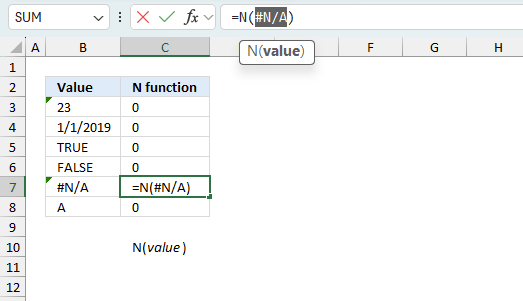
There is also another way to debug formulas using the function key F9. F9 is especially useful if you have a feeling that a specific part of the formula is the issue, this makes it faster than the "Evaluate Formula" tool since you don't need to go through all calculations to find the issue.

1. Enter Edit mode: Double-press with left mouse button on the cell or press F2 to enter Edit mode for the formula.
2. Select part of the formula: Highlight the specific part of the formula you want to evaluate. You can select and evaluate any part of the formula that could work as a standalone formula.
3. Press F9: This will calculate and display the result of just that selected portion.
4. Evaluate step-by-step: You can select and evaluate different parts of the formula to see intermediate results.
5. Check for errors: This allows you to pinpoint which part of a complex formula may be causing an error.

The image above shows cell reference B7 converted to hard-coded value using the F9 key. The N function requires non-error values as input values which is not the case in this example. We have found what is wrong with the formula.

Tips!

• View actual values: Selecting a cell reference and pressing F9 will show the actual values in those cells.
• Exit safely: Press Esc to exit Edit mode without changing the formula. Don't press Enter, as that would replace the formula part with the calculated value.
• Full recalculation: Pressing F9 outside of Edit mode will recalculate all formulas in the workbook.

Remember to be careful not to accidentally overwrite parts of your formula when using F9. Always exit with Esc rather than Enter to preserve the original formula. However, if you make a mistake overwriting the formula it is not the end of the world. You can “undo” the action by pressing keyboard shortcut keys CTRL + z or pressing the “Undo” button

6.3 Other errors

Floating-point arithmetic may give inaccurate results in Excel - Article

Floating-point errors are usually very small, often beyond the 15th decimal place, and in most cases don't affect calculations significantly.

Functions in 'Information' category

The N function function is one of 19 functions in the 'Information' category.

Excel function categories

Excel categories

Leave a Comment