How to use the EOMONTH function

What is the EOMONTH function?

The EOMONTH function returns an Excel date for the last day of a given month using a number and a start date. Use EOMONTH to calculate maturity dates or due dates that fall on the last day of the month.

1. Introduction

What is EOMONTH an abbreviation of?

EOMONTH stand for End Of month.

What are dates in Excel?

Dates are stored numerically but formatted to display in human-readable date/time formats, this enables Excel to do work with dates in calculations.

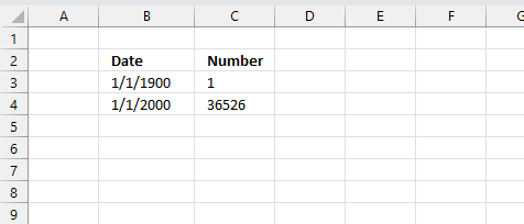
For example, dates are stored as sequential serial numbers with 1 being January 1, 1900 by default. The integer part (whole number) represents the date the decimal part represents the time.

This allows dates to easily be formatted to display in many date/time formats  like mm/dd/yyyy, dd/mm/yyyy and so on and still be part of calculations as long as the date is stored numerically in a cell.

You can try this yourself, type 10000 in a cell, press CTRL + 1 and change the cell's formatting to date, press with left mouse button on OK. The cell now shows 5/18/1927.

What is a maturity date?

The maturity date is the date on which the principal amount of a security becomes due and payable to the holder. It applies to fixed-income securities like bonds, notes, bills where the issuer must repay the principal on the maturity date.

At maturity, the debt is fully repaid. The security might cease to exist after maturity. Maturity dates affect interest rate risk - longer terms have higher risk. The final coupon payment is made on the maturity date.

What is a due date?

The due date is the date on which a debt payment is due to be paid by a borrower to a lender. It applies to loans, mortgages, credit cards, accounts receivables where periodic payments are required.

A due date recurrence can be monthly, quarterly, annually based on the terms. Missing a due date can result in late fees or interest charges.

Related functions

Excel Function	Description
DATEDIF(start_date, end_date, unit)	Returns the time between two dates in specified units like complete years or months
EDATE(start_date, months)	Returns the date that is the indicated number of months before or after start_date
EOMONTH(start_date, months)	Returns the last day of the month before or after start_date by months
MONTH(date)	Returns the month of a date (1-12)
DATE(year, month, day)	Returns an Excel date

2. Syntax

EOMONTH(start_date, months)

start_date	Required. A date that represents the starting date. Don't use text dates, use Excel dates, see comments below.
months	Required. A number that determines how many months before or after the start date. A negative value returns a date earlier than the start_date.

3. Example

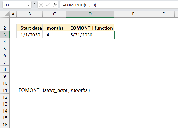
The image above shows the EOMONTH function cell D3 calculating the last day of the month based on a start date specified in cell B3 and the number of months specified in cell C3.

Formula in cell D3:

The function calculates 5/31/2030 based on the start date 1/1/2030 and add 4 months to that. The last day in May 2030 is 31.

4. Calculate quarterly dates for the last day of a given month

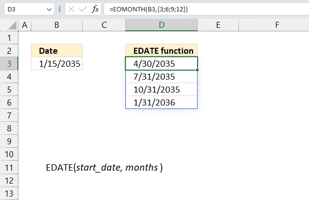
This example demonstrates how to calculate four different dates in the same calculation using arrays in Excel. The calculated dates are exactly three months a part from the start date and is the last date in that particular month.

Formula in cell D3:

{3;6;9;12} is an array of numbers separated by a semicolon. Excel performs four different calculations in the same cell and returns an array to cell D3 and the cells below as far as needed. This is called spilling and is a new feature in Excel 365.

5. Calculate bi monthly dates for the last day of a given month

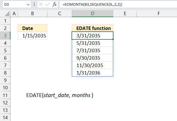
This example demonstrates how to calculate six different dates in the same calculation using arrays in Excel. The calculated dates are exactly two months a part from the start date and is the last date in that particular month.

Formula in cell D3:

Explaining formula in cell D3

Step 1 - Create a sequence from 2 to 12 with step 2

The SEQUENCE function creates a list of sequential numbers.

Function syntax: SEQUENCE(rows, [columns], [start], [step])

SEQUENCE(6,,2,2)

returns

{2;4;6;8;10;12}

Step 2 - Calculate dates

EOMONTH(B3,SEQUENCE(6,,2,2))

becomes

EOMONTH(B3,{2;4;6;8;10;12})

and returns

{49399;49460;49521;49582;49643;49705}.

6. EOMONTH function tips

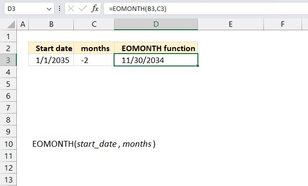
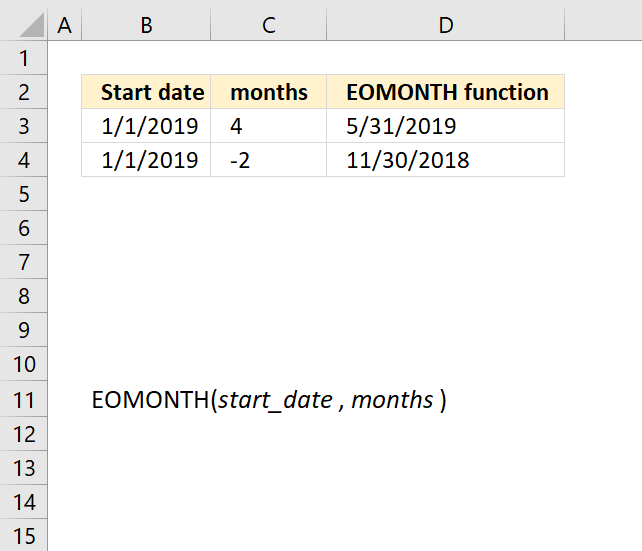
Use a negative number as the month argument to get a date before the start date. The image above shows the start date in cell B3, -2 in cell C3 which represents the month argument and the result in cell D3.

1/1/2035 minus two months is November 2034 and the last date in that month is 11/30/2034.

7. EOMONTH function not working

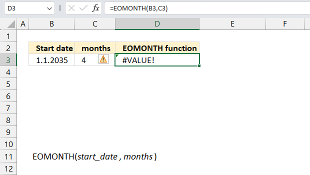
An invalid date demonstrated in cell B5 returns a #VALUE! error displayed in cell D5. Use the method explain here to convert invalid dates to dates that work: DATEVALUE function The EOMONTH function truncates a decimal value representing the months argument.

What is truncate? Removing the decimal leaving only the whole number. For example, truncate 7.9 and you get 7.

7.1 Troubleshooting the error value

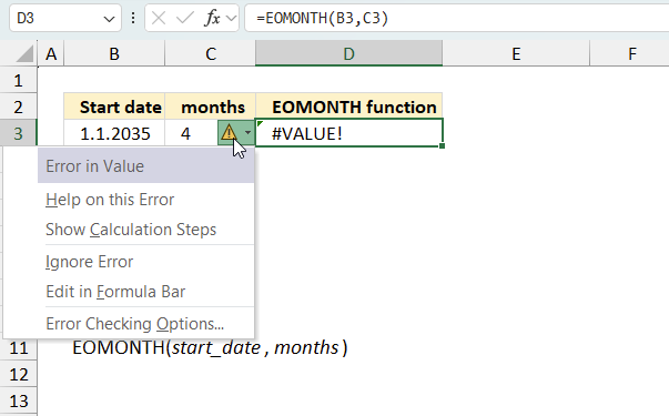
When you encounter an error value in a cell a warning symbol appears, displayed in the image above. Press with mouse on it to see a pop-up menu that lets you get more information about the error.

1. The first line describes the error if you press with left mouse button on it.
2. The second line opens a pane that explains the error in greater detail.
3. The third line takes you to the "Evaluate Formula" tool, a dialog box appears allowing you to examine the formula in greater detail.
4. This line lets you ignore the error value meaning the warning icon disappears, however, the error is still in the cell.
5. The fifth line lets you edit the formula in the Formula bar.
6. The sixth line opens the Excel settings so you can adjust the Error Checking Options.

Here are a few of the most common Excel errors you may encounter.

#NULL error - This error occurs most often if you by mistake use a space character in a formula where it shouldn't be. Excel interprets a space character as an intersection operator. If the ranges don't intersect an #NULL error is returned. The #NULL! error occurs when a formula attempts to calculate the intersection of two ranges that do not actually intersect. This can happen when the wrong range operator is used in the formula, or when the intersection operator (represented by a space character) is used between two ranges that do not overlap. To fix this error double check that the ranges referenced in the formula that use the intersection operator actually have cells in common.

#SPILL error - The #SPILL! error occurs only in version Excel 365 and is caused by a dynamic array being to large, meaning there are cells below and/or to the right that are not empty. This prevents the dynamic array formula expanding into new empty cells.

#DIV/0 error - This error happens if you try to divide a number by 0 (zero) or a value that equates to zero which is not possible mathematically.

#VALUE error - The #VALUE error occurs when a formula has a value that is of the wrong data type. Such as text where a number is expected or when dates are evaluated as text.

#REF error - The #REF error happens when a cell reference is invalid. This can happen if a cell is deleted that is referenced by a formula.

#NAME error - The #NAME error happens if you misspelled a function or a named range.

#NUM error - The #NUM error shows up when you try to use invalid numeric values in formulas, like square root of a negative number.

#N/A error - The #N/A error happens when a value is not available for a formula or found in a given cell range, for example in the VLOOKUP or MATCH functions.

#GETTING_DATA error - The #GETTING_DATA error shows while external sources are loading, this can indicate a delay in fetching the data or that the external source is unavailable right now.

7.2 The formula returns an unexpected value

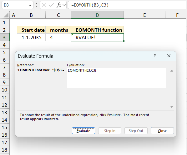
To understand why a formula returns an unexpected value we need to examine the calculations steps in detail. Luckily, Excel has a tool that Here is how to troubleshoot a formula:

1. Select the cell containing the formula you want to examine in detail.
2. Go to tab “Formulas” on the ribbon.
3. Press with left mouse button on "Evaluate Formula" button. A dialog box appears.
   The formula appears in a white field inside the dialog box. Underlined expressions are calculations being processed in the next step. The italicized expression is the most recent result. The buttons at the bottom of the dialog box allows you to evaluate the formula in smaller calculations which you control.
4. Press with left mouse button on the "Evaluate" button located at the bottom of the dialog box to process the underlined expression.
5. Repeat press with left mouse button oning the "Evaluate" button until you have seen all calculations step by step. This allows you to examine the formula in greater detail and hopefully find the culprit.
6. Press "Close" button to dismiss the dialog box.

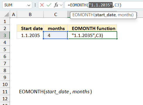
There is also another way to debug formulas using the function key F9. F9 is especially useful if you have a hunch that a specific part of the formula is the issue, this makes it faster than the "Evaluate Formula" tool since you don't need to go through all calculations to find the issue..

1. Enter Edit mode: Double-press with left mouse button on the cell or press F2 to enter Edit mode for the formula.
2. Select part of the formula: Highlight the specific part of the formula you want to evaluate. You can select and evaluate any part of the formula that could work as a standalone formula.
3. Press F9: This will calculate and display the result of just that selected portion.
4. Evaluate step-by-step: You can select and evaluate different parts of the formula to see intermediate results.
5. Check for errors: This allows you to pinpoint which part of a complex formula may be causing an error.

The image above shows cell reference B3 converted to hard-coded value using the F9 key. The hardcoded value is a text string and the EOMONTH function expects a number representing the Excel date. We have found what is wrong with the formula using the F9 key.

Tips!

• View actual values: Selecting a cell reference and pressing F9 will show the actual values in those cells.
• Exit safely: Press Esc to exit Edit mode without changing the formula. Don't press Enter, as that would replace the formula part with the calculated value.
• Full recalculation: Pressing F9 outside of Edit mode will recalculate all formulas in the workbook.

Remember to be careful not to accidentally overwrite parts of your formula when using F9. Always exit with Esc rather than Enter to preserve the original formula. However, if you make a mistake overwriting the formula it is not the end of the world. You can “undo” the action by pressing keyboard shortcut keys CTRL + z or pressing the “Undo” button

Other errors

Floating-point arithmetic may give inaccurate results in Excel - Article

Floating-point errors are usually very small, often beyond the 15th decimal place, and in most cases don't affect calculations significantly.

8. EOMONTH function alternative

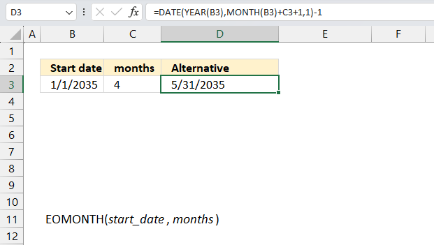
This example demonstrates an alternative way to calculate the end of month date using a formula instead of the EOMONTH function. Cell B3 contains an Excel date which is 1/1/2035, cell C3 contains 4 meaning 4 months.

Formula in cell D3:

The formula in cell D3 returns 5/31/2035 which is the last date in May based on adding 4 months to  1/1/2035.

Explaining formula in cell D3

Step 1 - Calculate the year

The YEAR function converts a date to a number representing the year in the date.

Function syntax: YEAR(serial_number)

YEAR(B3)

becomes

YEAR(49310)

and returns "2035".

Step 2 - Calculate the month

The MONTH function extracts the month as a number from an Excel date.

Function syntax: MONTH(serial_number)

MONTH(B3) +C3 + 1

becomes

MONTH(49310) + 4 + 1

becomes

1 + 4 + 1

and returns 6.

Step 3 - Calculate the Excel date

The DATE function returns a number that acts as a date in the Excel environment.

Function syntax: DATE(year, month, day)

DATE(YEAR(B3),MONTH(B3)+C3+1,1)

becomes

DATE(2035,6,1)

and returns "6/1/2035" (49460)

Step 4 - Subtract Excel date by 1

DATE(YEAR(B3),MONTH(B3)+C3+1,1) - 1

becomes

49460 - 1

and returns

49459 (5/31/2035)

'EOMONTH' function examples

Functions in 'Date and Time' category

The EOMONTH function function is one of 22 functions in the 'Date and Time' category.

Excel function categories

Excel categories

Comments (3)