How to use the AMORLINC function

What is the AMORLINC function?

The AMORLINC function calculates the depreciation for each accounting period. This function is designed for the French accounting system. The prorated depreciation is taken into account if an asset is bought in the middle of the accounting period.

AMORLINC is an abbreviation for “Amortissement linéaire” which means “linear depreciation” in French.

1. Introduction

What is depreciation?

Depreciation is an accounting method that allows businesses to allocate the cost of a tangible asset over its useful life. It represents how much of an asset’s value has been used up over time.

Depreciation helps businesses to match their expenses with their revenues, and to reduce their taxable income by deducting the depreciation expense.

What is an accounting period?

An accounting period is a span of time that covers certain accounting functions such as recording transactions etc. Some common types of periods are: Calendar year, fiscal year, and interim periods.

What is salvage value?

Salvage value is the estimated value of an asset at the end of its useful life. It is also known as scrap value or residual value. It is used to calculate the depreciation expense of an asset over its useful life.

What is prorated depreciation?

Prorated depreciation is a way of calculating the depreciation expense of an asset based on the proportion of time it is used in a given period. Prorated depreciation is often used when an asset is acquired or disposed of in the middle of an accounting period, and the depreciation method depends on the number of years or months of service. Prorated depreciation allows the business to match the expense of the asset with the revenue it generates more accurately.

2. Syntax

AMORLINC(cost, date_purchased, first_period, salvage, period, rate, [basis])

cost	Required.
date_purchased	Required.
first_period	Required. The date of the end of the first period.
salvage	Required. The salvage value.
period	Required.
rate	Required. The rate of depreciation.
[basis]	Required. The year count.

Basis	Day count
0 (default)	360 (NASD)
1	Actual
3	365
4	European 360

The depreciation rate will grow to 50 percent for the period before the last period and grows to 100 percent for the last period.

Comments

The prorated depreciation is taken into account if an asset is purchased in the middle of the accounting period.

Keep in mind to use the DATE function if you enter dates in the function instead of using cell references.

For example,

3. Example 1

A company purchases equipment for $3600 with a salvage value of $500. Calculate the depreciation for the first period using the depreciation rate of 20%?

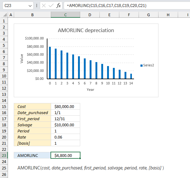
The arguments are:

• cost = 80000
• date_purchased = 45292
• first_period = 45657
• salvage = 10000
• period = 1
• rate = 0.06 (6%)
• [basis] = 1

Formula in cell C23:

The formula returns 4800 which represents the depreciation for period 1. The chart above shows the depreciation across periods until the salvage value is reached.

4. Example 2

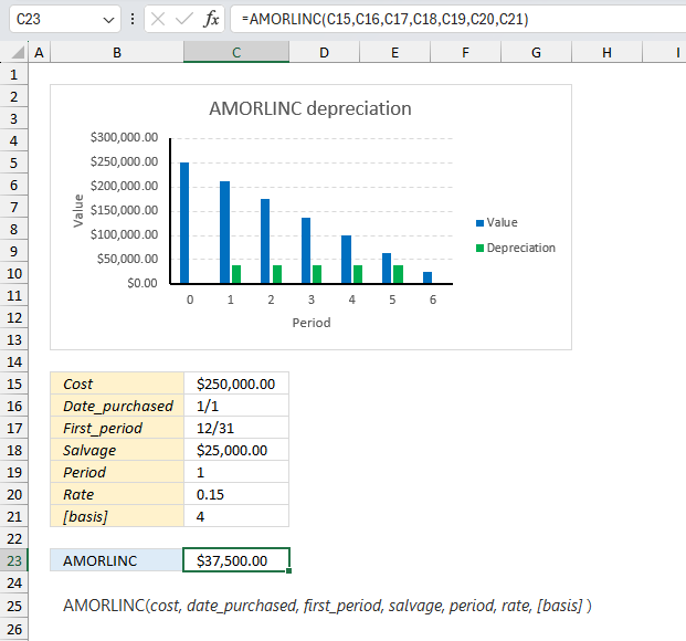
An asset with a cost of $250,000, a salvage value of $25,000, has a depreciation rate of 15%. The date purchased is 1/1 and the first period ends at 12/31. Use the European 360 day count. Determine the depreciation for period 1?

The arguments are:

• cost = 250000
• date_purchased = 45292
• first_period = 45657
• salvage = 25000
• period = 1
• rate = 0.15 (15%)
• [basis] = 4

Formula in cell C23:

The formula returns 37500 which represents the depreciation for period 1. The chart above shows the depreciation across periods until the salvage value is reached.

5. Example 3

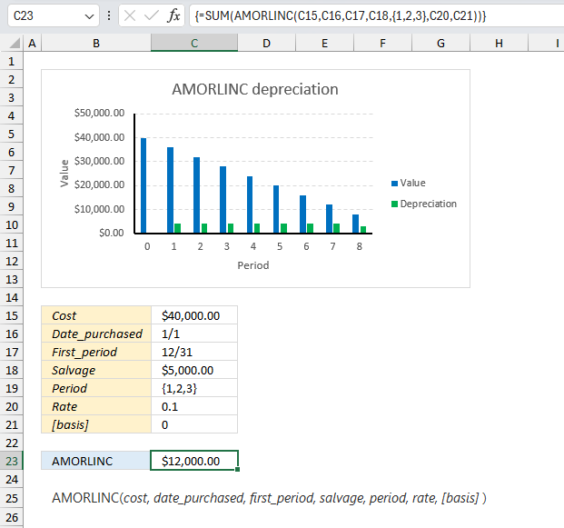
A vehicle was acquired for $40,000 with an estimated salvage value of $5,000, has a depreciation rate of 10%. The date purchased is 1/1 and the first period ends at 12/31. Calculate the total depreciation after three periods.

The arguments are:

• cost = 40000
• date_purchased = 45292
• first_period = 45657
• salvage = 5000
• period = {1,2,3}
• rate = 0.10 (10%)
• [basis] = 0

Array formula in cell C23:

The formula returns 12000 which represents the total depreciation for period 1, 2, and 3. The chart above shows the depreciation across periods until the salvage value is reached.

Explaining formula

Step 1 - Determine periods

We want to calculate the depreciation for periods 1, 2, and 3, to accomplish that we can use curly brackets to specify three different constants: {1,2,3}

This requires us to enter the formula as an array formula. Excel 365 subscribers may enter the formula as a regular formula.

Step 2 - Specify arguments

The arguments are specified in cell range C15:C21 except for the array containing the constants. They must be entered in the formula and not in the worksheet.

AMORLINC(C15,C16,C17,C18,{1,2,3},C20,C21)

becomes

AMORLINC(40000,45292,45657,5000,{1,2,3},0.1,0)

Step 3 - Add all calculations and return a total

The SUM function allows you to add numerical values, the function returns the sum in the cell it is entered in. The SUM function is cleverly designed to ignore text and boolean values, adding only numbers.

Function syntax: SUM(number1, [number2], ...)

SUM(AMORLINC(C15,C16,C17,C18,{1,2,3},C20,C21))

becomes

SUM({4000,4000,4000})

and returns 12000.

6. Example 4

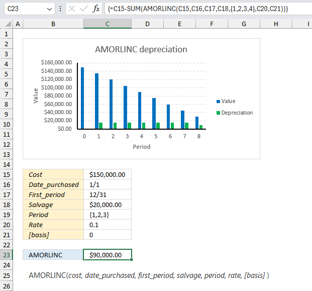
A business invests in machinery costing $150,000 with an estimated salvage value of $20,000. What is the value left after 3 periods?

The arguments are:

• cost = 150000
• date_purchased = 45292
• first_period = 45657
• salvage = 20000
• period = {1,2,3}
• rate = 0.10 (10%)
• [basis] = 0

Array formula in cell C23:

The formula returns 90,000 which represents the value left after three periods. The chart above shows the depreciation across periods until the salvage value is reached.

Explaining formula

Step 1 - Determine periods

We want to calculate the depreciation for periods 1, 2, 3, and 4, to accomplish that we can use curly brackets to specify three different constants: {1,2,3,4}

This requires us to enter the formula as an array formula. Excel 365 subscribers may enter the formula as a regular formula.

Step 2 - Specify arguments

The arguments are specified in cell range C15:C21 except for the array containing the constants. They must be entered in the formula and not in the worksheet.

AMORLINC(C15,C16,C17,C18,{1,2,3,4},C20,C21)

becomes

AMORLINC(150000,45292,45657,20000,{1,2,3,4},0.1,0)

and returns {15000,15000,15000,15000}

Step 3 - Add all calculations and return a total

The SUM function allows you to add numerical values, the function returns the sum in the cell it is entered in. The SUM function is cleverly designed to ignore text and boolean values, adding only numbers.

Function syntax: SUM(number1, [number2], ...)

SUM(AMORLINC(C15,C16,C17,C18,{1,2,3},C20,C21))

becomes

SUM({15000,15000,15000,15000})

and returns 60000.

Step 4 - Subtract cost with 4 periods of depreciation

The minus character lets you calculate the difference between two numerical values. In this particular example, the original cost minus the total of 4 periods of depreciation equals what is left of the value of the machinery.

C15-SUM(AMORLINC(C15,C16,C17,C18,{1,2,3,4},C20,C21))

becomes

150000-60000 equals 90000

Functions in 'Financial' category

The AMORLINC function function is one of 27 functions in the 'Financial' category.

Excel function categories

Excel categories

Leave a Comment