How to use an Excel Table name in Data Validation Lists and Conditional Formatting formulas – use named ranges
This article demonstrates different ways to reference an Excel defined Table in a drop-down list and Conditional Formatting formulas. The issue is that you can't use structured references. There are two workarounds, the INDIRECT function or a named range. I will, in this article, explain the advantages and draw-backs of each workaround.
Table of Contents
1. Introduction
What is a cell reference?
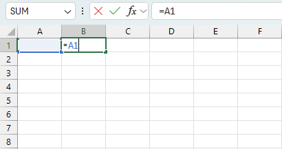
A cell reference is the way to identify a specific cell or range of cells in a spreadsheet such as A1 which refers to column A row 1. The purpose of the cell reference is to get the value from the given cell which you can use to calculate a new value or whatever you have in mind.
Cell references is mostly used in formulas but built-in features like conditional formatting or drop-down-lists etc. may also use cell refs. Cell references has three different states:
- Relative cell ref: For example, A1. The cell ref changes when copied or moved.
- Absolute cell ref: For example, $A$1. Remains fixed when the cell is copied and then pasted to a new cell.
- Mixed cell ref: For example, $A1 or A$1. Partially fixed meaning either the column or the row remains the same. The position of the dollar sign determines if the column or row is fixed.
Here is how to create a cell reference:
- Double press with left mouse button on a specific cell to start typing.For example, B1.
- Type = and then the cell reference, for example =A1
This creates a cell reference in cell B1 that points to cell A1.
What is a structured reference?
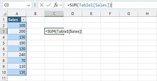
A structured reference is a way to refer to table data using table names and column headers instead of traditional cell references. Example:
- =Table1[Sales] refers to the "Sales" column in "Table1".
- =SUM(Table1[Sales]) calculates the sum of all values in the "Sales" column.
The great advantage of using structured references is that the structured cell reference does not change when new values are added or deleted compared to regular cell references. For example:
Imagine that Table1[Sales] is equivalent to cell range A1:A10.
- A formula that sums these values using regular cell references looks like this: =SUM(A1:A10)
This formula must be changed if the cell range grows or shrinks. For example, a new value is added to cell A11. The formula is now: =SUM(A1:A11) - A formula that sums these values using a structured cell reference looks like this: =SUM( Table1[Sales] )
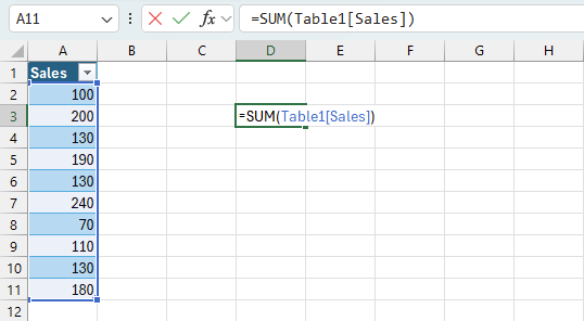
What happens if we add a new value in cell A11? The Excel defined Table automatically includes the new value and the strucutred cell reference stays the same: =SUM( Table1[Sales] )
This works only if you add values adjacent to the Excel defined Table.
What is a volatile function?
A volatile function is a function that recalculates each time the worksheet recalculates. A regular function calculates only when the formula is entered. This means that all volatile functions recalculate when a new value or formula is entered in a cell on the same worksheet. The default setting in Excel is to recalculate the worksheet, you can find the setting here:
- Go to tab "Formulas" on the ribbon.
- Press with left mouse button on with the left mouse button "Calculations Options" button. A popup menu appears. See the image below.
- Select the preferred setting.
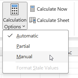
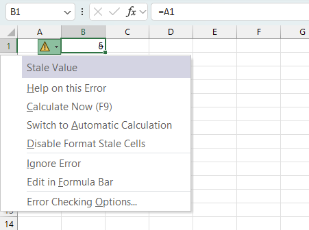
If you change the calculation options to manual, you must press F9 to recalculate the worksheet formulas. This allows you to control when the intensive cpu calculations are made. Excel 365 lets you know when you have stale values by applying strike-through formatting demonstrated in cell B1 in the image below.
The INDIRECT function is a volatile function meaning it recalculates every time Excel recalculates which is not the case with most Excel functions. Using this function in Excel extensively can significantly slow down the calculations in your workbook.
It is a powerful function but it can be computationally intensive, especially when used repeatedly or in complex formulas. It's important to be cautious when using the INDIRECT function as it may have a noticeable impact on the performance and responsiveness of your Excel workbook.
What to do if the worksheet calculations are slow?
If you find that your workbook is running slowly or calculations are taking a long time to complete, the overuse of volatile functions may be a contributing factor. As I see it you have two options:
- Replace volatile functions with non-volatile functions if possible.
- Control when the calculations are made.
See the instructions above on how to enable manual calculations and use F9 to control calculations.
What is a hard-coded formula?
Another downside with the function apart from being volatile is that the Excel Table name is "hard-coded" into the formula. This means that the formula will stop working if you change the Excel Table name.
Here is how to edit a conditional formatting formula:
- Select the cells which have the conditional formatting applied.
Here is how to change the name of a specific Excel defined Table:
- Select any cell in the specific Excel Table. A new tab named "Table design" appears on the ribbon.
What is an Excel defined Table?
What is conditional formatting?
Is Conditional Formatting volatile?
What is a named range?
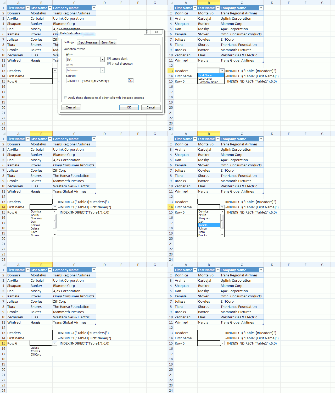
1. How to populate a drop-down list with Excel Table headers?
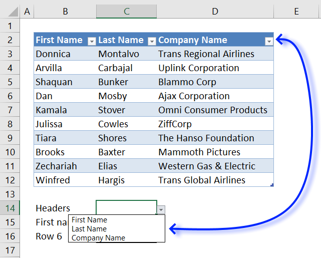
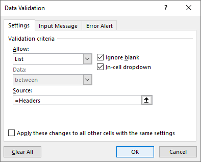
Drop-down lists is a data validation tool that allows you to control what the user enters in a given cell. Drop-down lists does not support references to Excel Tables, we need a workaround. You have two options, that I will demonstrate below, the INDIRECT function or "Named ranges". The image above shows a drop-down list populated with Excel Table header values, this formula allows you to use Excel table headers as values in a drop-down list. The following formula shows how to use Excel Table references in drop-down lists:
The downside with this approach is that the formula is hard-coded meaning if you change the Excel Table name this formula still references the old name. You need to adjust this formula as well. You can also create a "named range" and reference the Excel Table headers there. The advantage with "Named ranges" is that it adjusts automatically if you change the name of the Excel Table to the new name which is not the case with the INDIRECT function.
- Go to tab "Formulas" on the ribbon.
- Press with left mouse button on "Name Manager" button to open the "Name Manager" dialog box.
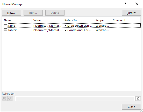
- Press with left mouse button on the "New" button.
- Type the reference, in this case: =Table1[#Headers]
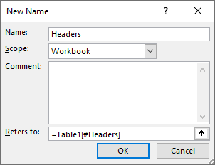
- Press with left mouse button on OK button.
- Press with left mouse button on Close button.
Now use the named range name Headers in the Data Validation dialog box.
1.1 Watch this video to learn more
2. How to populate a drop-down list with values from an Excel Table column?
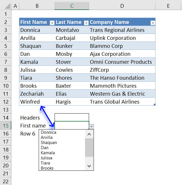
The easiest way is to use the INDIRECT function to create a reference to an Excel Table column. References pointing to an Excel Table are called "structured references", they are different from regular cell references. Structured references in Excel refer to the way you can refer to cells and ranges within an Excel table using a specific syntax.
- Referencing Cells: Instead of using traditional cell references like A1 or B5, structured references use the table name and column name, like TableName[@[ColumnName]]. The @ character in a structured reference in Excel is used to reference the current row within the table. When you use the @ symbol in a structured reference, it allows you to refer to the value in the current row for a specific column, rather than referencing a fixed row or the entire column. This allows you to create formulas or references that are relative to the current row, rather than being fixed to a specific row. This can be particularly useful when you want to perform calculations or comparisons within the context of the current row.
- Referencing columns: TableName[ColumnName].Referencing columns in Excel Tables using the structured reference format TableName[ColumnName] is a powerful way to work with data in your spreadsheets.
TableName: This is the name of the Excel Table that you're referencing. Tables in Excel are defined as a range of cells with a header row, and they have a unique name.
[ColumnName]:This is the name of the column within the Excel Table that you want to reference. Column names in Excel Tables are typically defined in the header row of the table. - Referencing Ranges: You can reference a whole range within a table using the table name and [#All] or [#Data] to refer to the entire table data.
TableName[#All] references all data in the Excel Table including the header names.
TableName[#Data] or simply TableName returns all data in the Excel Table excluding the header names.
Structured references make it easier to create calculated columns within a table, as the references automatically adjust when the table is expanded. Formulas that use structured references are more robust and flexible, as they can automatically adjust when the table structure changes. Structured references make formulas more self-documenting and easier to understand, as the column names provide context. Using structured references can help improve the maintainability and flexibility of your Excel workbooks, especially when working with large or complex data sets organized in tables. They provide a more intuitive and dynamic way to reference data compared to traditional cell-based references.
Cell B15 contains a drop-down list with this formula:
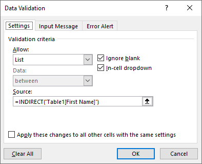
You can also use named ranges to reference a particular column:
- Go to tab "Formulas" on the ribbon.
- Press with left mouse button on "Name Manager" button to open the "Name Manager" dialog box.

- Press with left mouse button on the "New" button.
- Type the reference, in this case: =Table1[First Name]

(Note that the image above shows how to reference header names, not an Excel column) Change the name of the named range accordingly. - Press with left mouse button on OK button.
- Press with left mouse button on Close button.
Now use the named range name that you specified in step 4 above in the Data Validation dialog box.

3. How to populate a drop-down list with values from an Excel Table row?
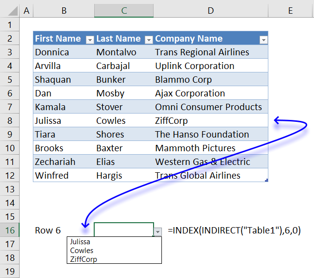
The INDEX function is capable of extracting values in a single row from a cell range, combine it with the INDIRECT function and a reference to the Excel Table, please see formula below.
Reference a table row in a drop down list, cell B15:
Animated image
The animated image above demonstrates the drop-down lists, how they work and what they link to.
4. How to reference an Excel Table in a Conditional Formatting formula?
Simply add the INDIRECT function to each Excel Table reference in your formula, please see formula below.
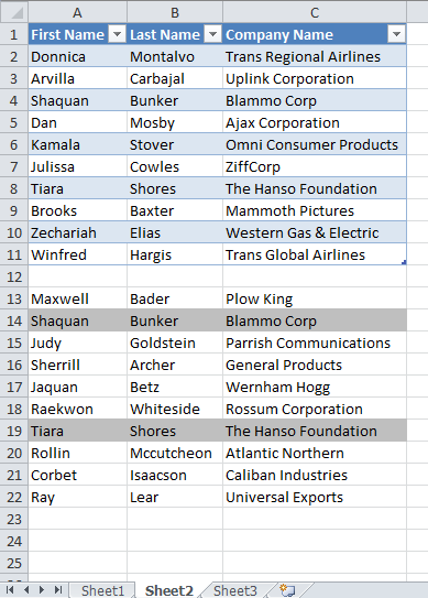
Conditional formatting formula, cell range A13:C22:
The Conditional Formatting formula highlights a row if a record in cell range A13:C22 is equal to at least one record in the Excel defined Table (A1:C11)
5. How to reference Excel 365 dynamic array formulas
Dynamic arrays are a powerful feature introduced in Excel 365 that automatically spill results into multiple cells when a formula returns more than one value. This is a significant change from how arrays worked in previous Excel versions. Let me explain the key differences:
Dynamic Arrays in Excel 365:
- Automatic spilling: Formulas that return multiple results automatically expand into neighboring cells.
- No need for Ctrl+Shift+Enter: You don't need to enter array formulas with a special key combination.
- Dynamic resizing: The result range automatically adjusts if the source data changes.
- New functions: Introduced several new functions like SORT, FILTER, UNIQUE, and SEQUENCE.
You can reference these formulas using the # symbol which is called the spill range operator. It refers to the entire dynamic array that starts in, for example, B5then you reference it like this: =B5#. This allows you to perform operations on the whole array without needing to specify the exact range.
The issue is that you can't reference a dynamic array formula in Drop-down lists, Charts, Pivot Tables and Conditional formatting. The preferred way, in my opinion, is to use "Named ranges" in order to reference dynamic array formulas in the features mentioned above.
Get the Excel file
Reference-a-table-in-a-data-validation-list-or-conditional-formatting-formula.xlsx
Data validation category
Table of Contents Create dependent drop down lists containing unique distinct values - Excel 365 Create dependent drop down lists […]
Question: How do I create a drop-down list with unique distinct alphabetically sorted values? Table of contents Introduction Sort values […]
Table of contents How to change cell formatting using a Drop Down list Highlight cells based on coordinates Highlight every […]
Drop down lists category
Table of Contents Create dependent drop down lists containing unique distinct values - Excel 365 Create dependent drop down lists […]
Question: How do I create a drop-down list with unique distinct alphabetically sorted values? Table of contents Introduction Sort values […]
Table of contents How to change cell formatting using a Drop Down list Highlight cells based on coordinates Highlight every […]
Table category
Table of Contents How to compare two data sets - Excel Table and autofilter Filter shared records from two tables […]
This article demonstrates two formulas that extract distinct values from a filtered Excel Table, one formula for Excel 365 subscribers […]
The image above demonstrates a macro linked to a button. Press with left mouse button on the button and the […]
How to use Excel Tables
32 Responses to “How to use an Excel Table name in Data Validation Lists and Conditional Formatting formulas – use named ranges”
Leave a Reply
How to comment
How to add a formula to your comment
<code>Insert your formula here.</code>
Convert less than and larger than signs
Use html character entities instead of less than and larger than signs.
< becomes < and > becomes >
How to add VBA code to your comment
[vb 1="vbnet" language=","]
Put your VBA code here.
[/vb]
How to add a picture to your comment:
Upload picture to postimage.org or imgur
Paste image link to your comment.




How would you replace [First Name] with the value of the chose header field?
it only seems to work when specifically selecting the Header name like [First Name]
id like it to be more dynamic.
if i chose Last Name in the headers dropdown, i would like to see Onlyl the Last Name Choices in the next dropdown box.
Ralf,
read this post:
Create dependent drop down lists containing unique distinct values
Thank you! This tip has saved me a whole lot of effort.
Chris Hills,
Thank you for commenting!
Hello,
i have a question.
It's possible "data validation" in collaboration mode, because is not work for me (2002, 2007)?
Therefore i think, then i creating a macro, that paste a "drop down list" into cells.
Thank You for Your answer
It's possible "data validation" in collaboration mode, because is not work for me (2002, 2007)?
No!
Avoiding Shared Workbooks in Excel
Thank You
This is great - love this overall approach as a framework for data validation as opposed to the old way of naming ranges but then having to use OFFSET + COUNT so that the ranges could expand/contract based on data in them.
My only question is, why does Excel require the INDIRECT when referring to these table properties during data validation in the first place? If I am typing a normal formula, I can just get refer directly to Table[Column1] as in =SUM(Table[Column1]. BUT, if I want to do data validation, I can't type in =Table[Column1] but have to instead wrap that in quotes and then use INDIRECT.
Why?
Jake,
My only question is, why does Excel require the INDIRECT when referring to these table properties during data validation in the first place? If I am typing a normal formula, I can just get refer directly to Table[Column1] as in =SUM(Table[Column1]. BUT, if I want to do data validation, I can't type in =Table[Column1] but have to instead wrap that in quotes and then use INDIRECT.
Only Microsoft can answer your question but my guess is that they have not thought this through.
Thanks for this ... just what I needed. Just hit the problem of a) not being able to use a table in Data Validation and b) not being able to use a table in Conditional Formatting. And here's the answer to both my problems in one go! Excellent.
I had worked around it by defining a Named Range and referring that to the data area of the table. I thought that was a neat little get out of jail card. *But* it seemed a little tedious having to use two references for one range.
So, thank you very much for your help. Trevor
Trevor,
thank you for commenting!
Oscar, you're really welcome. You would not believe how useful this has been in a current project. Hours of fun :)
So much easier than creating Dynamic Named Ranges (although I use INDEX/COUNTA rather than OFFSET)
Cheers and thanks again.
Thank You!!!!!
Is there a way of using the table reference as you have defined above but allowing for the fact that there may be blanks in one or more rows.
For instance in my table I might have 200 rows, but for my dropdown I only want to collect the non-blank row values. At the moment I end up with a lot of blanks in my dropwdown because of this issue. Haven't yet found a way round it..although it may be obvious!
Many thanks
Tony
The only way I have so far found to do it is using INDIRECT as follows:
=INDIRECT("Import!$X$2:$X$" & COUNTA(RawData[Currencies])-COUNTBLANK(RawData[Currencies]))
The COUNTA(...) - COUNTBLANK(..)
is required it would seem as COUNTA on its own will count cells with a formula in them even though the value is blank (""). COUNTBLANK counts blank cells even if there is a formula.
Tony
Tony,
Thank you for posting a workaround.
Is there a way, other than building a calculated cell and pointing to that, of using concatenated table cells in the data validation list, using indirect? I've tried it, and it comes back with an error:
=INDIRECT("BReq_T[BR'#]") & " - " & INDIRECT("BReq_T[BR Scope]") & ": " & INDIRECT("BReq_T[BR Details]")
In short - I have two sheets - BReq (contains a list of Business Requirements) and FReq (contains a list of Functional Requirements).
Each FR is to be mapped to a number of BRs - but as the list contains BRs from across a number of phases, we need to ensure the user can determine that they are mapping the right BR, but without restricting the list - hence the concatenated list.
I can build a lookup list, and point data validation at that, but it is not ideal - so I thought the indirect method would work nicely, but alas it appears not in my case!
Any help would be appreciated - can send a sample workbook if needed.
Thank you!
Hi Oscar - I managed to sort this out using VBA and the SPLIT function - thanks.
Can you use the '=INDIRECT("PivotTable[Row FieldName]")' approach for validation when your data source is a Pivot table? It also seems to resolve in an error!
Thanks, Chris
[…] data validation from table column → […]
Thank you !
I have a table that has a list of employees and the columns include name, location, address, telephone #, etc... On another worksheet I have a list which lists each location, pick up person (must be employee) who will pick up paperwork that week. I only need 1 person from each location. Right now I have that as a data validation using the indirect function which lists all of the employees for me to choose from. I would like a data validation formula that looks at the employee info sheet and only shows me the ones that are from that location when I press with left mouse button on it.
Thanks for any advice!
good article... simply explained.
I'll come back for more tips...
This is an older post - so hoping someone will read this.
Indirects are powerful functions, but they come at a cost. Being a volatile function, they are always recalculated (and dependencies) whenever Excel needs to recalculate.
My question: what are the performance implications of using this method on a large workbook where efficiency is a must?
Hi, what if I have several people under the same company? For instance, I would like to choose a company first, let's say Trans Regional Airlines. But in Trans Regional Airlines, I usually talk to five people. I want to be able to pick one of the five people from the company through a list too. How can I do that?
I forget about INDIRECT. Great post.
Fantastic post, I know Named Ranges, I know Data Validation, I know Tables.
I know using a Named Range with spaces essentially breaks the Validation Part of a Drop Down.
However I didn't know to use a combination of Tables with Drop Down & Data Validation to make Excel actually fully usable!!
Thank you very much!!!
Hello Oscar
Thank you for the information, it was helpful. Can you please tell if it is possible to select multiple values using a table for data validation? Like in your example in a data-validated column is it possible to have values: Donnica, Arvilla
Excelent article. Is there a way to refer only to filtered table values in the list? It now seems that all the table field values appear in the drop down list regardless if table is filtered or not.
giedrius
This array formula lists all filtered values in column [First Name]:
=INDEX(Table1[First Name], SMALL(IF(SUBTOTAL(3, OFFSET(Table1[First Name], MATCH(ROW(Table1[First Name]), ROW(Table1[First Name]))-1, 0, 1)), MATCH(ROW(Table1[First Name]), ROW(Table1[First Name])),""),ROW(A1)))
However this won't work in a drop down list, only the first value in the array is shown.
Thank you very much, Oscar. A real time saver.
It is valuable information, indeed.
This is brilliant, but yeah, the only problem is that INDIRECT, especially multiple of them totally slows down a spreadsheet. I added into only one conditional format out of at least 2-dozen in a 2mb spreadsheet, and it jumped to 4mb for just one use conditional formatting formula.
You could try this formula in your Validation Source:
=OFFSET(tables!$A$2;0;0;COUNTA(tables!A:A)-1;1)
where your table is in tables!A:A