Auto resize columns as you type
Have you ever wanted Excel to react automatically when something changes in your spreadsheet? With Event Code in VBA you can make that happen! Event code allows Excel to respond to actions, such as entering data, press with left mouse button oning a cell, or filtering data. This can save time, reduce errors, and improve efficiency in your daily tasks.
In this article, we will explore four useful examples of event code that can make your Excel experience smoother and more powerful. Whether you're a beginner or have some VBA knowledge, these examples will help you understand how events work and how they can automate your workflow.
- Resize columns. The first example shows how to resize columns automatically. No need for the user to adjust column widths.
- Hide column.This example displays how to hide a given column if a specific cell is selected.
- Hide columns based on user input. The worksheet filters columns based on what values the user enter.
- Hide columns in an Excel Table. This example demonstrates how to hide columns in an Excel Table based on the selected drop down value, this changes the data which instantly updates a chart.
Let’s get started!
What's on this page
1. Introduction
What is VBA?
VBA (Visual Basic for Applications) is a programming language developed by Microsoft that is used for automating tasks in Microsoft Office applications such as Excel, Word, and Access. It allows users to create macros, automate repetitive tasks, and enhance Office functionality with custom scripts.
What is a macro?
In Microsoft Excel, a macro is a sequence of instructions written in Visual Basic for Applications (VBA) that allows you to automate repetitive tasks time consuming tedious tasks. Macros can perform a wide range of actions from simple formatting changes to complex data manipulations.
What is an event?
An event in Excel refers to an action or occurrence that triggers the execution of a specific macro. Events can be user-initiated, such as opening a workbook, changing a cell's value, or press with left mouse button oning a button, or system-initiated, like recalculating a worksheet. By associating macros with events users can automate responses to specific actions within the workbook.
What is event code?
Event code is placed in specific object modules like ThisWorkbook or a worksheet module (Sheet1, Sheet2). Regular VBA code is typically stored in a standard VBA module like Module1, Module2, etc...
What is an *.xlsm file?
Older Excel versions saved Excel files using the *.xls as the file extension. It was also possible to save VBA code in an *.xls file which made them potentially unsafe.
Excel 2007 introduced *.xlsx and *.xlsm files which made it safer to use Excel files. An *.xlsx file cant contain VBA code at all making them safer to use in contrast to older *.xls files
An .xlsm file is a type of Excel workbook that also supports macros which are automated scripts written in VBA which *.xlsx don't do. They use the Open XML format and differ from standard .xlsx files because they can store and run macros. This feature extends the capabilities of worksheets allowing you to automate processes and improve spreadsheet functionality. It's important to exercise caution when handling .xlsm files from untrusted sources as macros can contain code that may pose security risks.
2. Auto resize columns as you type
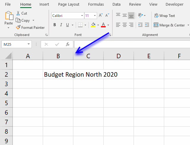
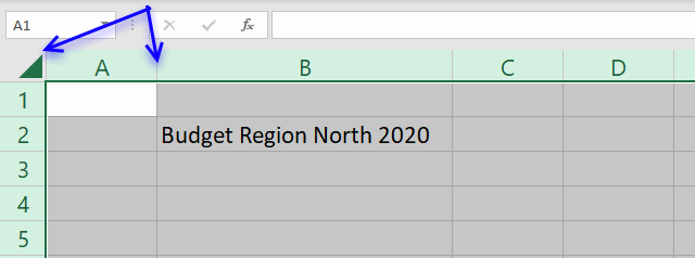
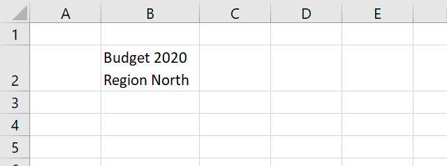
Excel does not resize columns as you type by default as the image above demonstrates. You can easily resize all columns manually by press with left mouse button oning on the column header next to column A and then double press with left mouse button on with left mouse button on any of the delimiting column lines.
Double-press with left mouse button oning on the column next to column A selects all cells on the worksheet, double-press with left mouse button oning on any of the delimiting column lines resizes all columns containing data so it fits accordingly.
You can also press short-cut keys CTRL + A in order to select all cells on the worksheet. Note that the selected cell must be empty before you press CTRL + A. If not, a cell range containing contiguous adjacent non-empty cells will be selected.
There is a short-cut for auto adjusting column widths as well, simply press Alt + H + O + I. Make sure you have selected the cells you want to to auto adjust before pressing the short-cut keys.
You can, however, create an Event that does this for you automatically. Let me show you how to create self-adjusting columns in Excel with a few lines of VBA code.
Example,
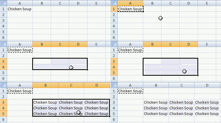
You can also copy and paste cells and the columns resize instantly.
Example,
The Event code displayed below is not placed in a regular code module, this event code is placed in the Workbook module, event code is rund when a specific thing happens.
For example, a cell is selected, a worksheet is activated, a workbook is closed, a cell value has changed etc. All these actions can trigger an Event, which Event is determined by the name of the macro.
2.1 VBA code
'The WorkbookSheetChange event is run if any of the cells in the workbook changes
Private Sub Workbook_SheetChange(ByVal Sh As Object, ByVal Target As Range)

'Don't show changes made to the worksheet
Application.ScreenUpdating = False

'Go through each cell that has been changed
For Each Value In Target.Columns

'Auto resize column using the Autofit method
    Worksheets(Sh.Name).Columns(Value.Column).AutoFit

'Continue with next cell that has changed
Next Value

'Show changes to the user
Application.ScreenUpdating = True

End Sub
The Target parameter is a range object containing the cell or cells that have been changed, the Sh parameter contains the worksheet object of the changed cells.
The ScreenUpdating property allows you to perform changes to the workbook without showing the result until all changes have been made, this makes the code run faster and smoother.
2.2 Where to copy code?
- Press Alt + F11 to open the VBA Editor.
- Double-press with left mouse button on ThisWorkbook in Project Explorer
- Copy VBA code
- Paste to the code module
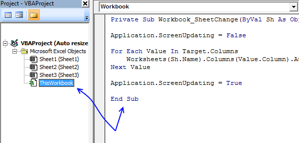
- Exit VBA editor and return to Excel
2.3 Final thoughts
The downside with this approach is that you lose the ability to undo any changes you make, there is, however, a solution to that: Generic undo routine for VBA
If you want to use two lines in one cell simply press Alt+Enter where you want the text to be split.
3. Press with left mouse button on a cell to make a column hidden or visible - VBA
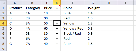
This example demonstrates how to build a macro that hides/shows a specific column if a given cell is selected. Each time the cell is selected the column toggles between visible/hidden.
The image above shows an example that hides/shows column E if any cell in column D is selected. This is made possible using Event code which is somewhat different than regular VBA code.
Event code is stored in a worksheet or workbook module instead of a regular code module, I will show you in detail how it works.
3.1 Event code
'Event code
Private Sub Worksheet_SelectionChange(ByVal Target As Range)

'Check if any cell in column D is selected and that only one cell in column D is selected
If Not Intersect(Target, Range("D:D")) Is Nothing And Target.Cells.CountLarge = 1 Then

    'Check if column e is hidden
    If Range("E:E").EntireColumn.Hidden = True Then

        'Show column E
        Range("E:E").EntireColumn.Hidden = False

    'Continue here if column E is visible
    Else

        'Hide column E
        Range("E:E").EntireColumn.Hidden = True
    End If
End If
End Sub
3.2 Where to put the event code?
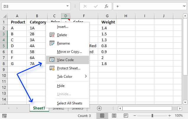
- Press with right mouse button on on the worksheet name, see image above.
- Press with left mouse button on "View Code". Visual Basic Editor opens, see image below.
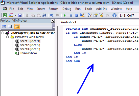
- Paste code to the worksheet module. The arrow in the image above shows where to put the event code.
- Exit VB Editor and return to Excel.
3.3 Animated image
3.4 Press with left mouse button on a button to hide/show a column

The animated image above shows that you can press with left mouse button on a button that runs a macro to hide or show a given column. This macro is saved in a regular module.
The button is a Form Control that you can easily create from the Developer tab, I will show you how later in this article.
3.5 VBA code
'Name macro
Sub HideColumn()

'Check if column F is hidden
If Range("F:F").EntireColumn.Hidden = True Then

    'Show column F
    Range("F:F").EntireColumn.Hidden = False

'Continue here if column F is visible
Else

    'Hide column F
    Range("F:F").EntireColumn.Hidden = True
End If

End Sub
3.6 Where to put the macro code?
- Copy above VBA code.
- Press shortcut keys Alt + F11 to open the Visual Basic Editor (VBE).
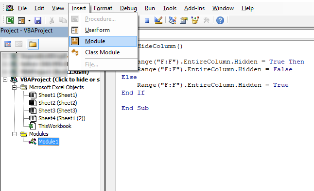
- Press with left mouse button on "Insert" on the top menu, see image above.
- Press with left mouse button on "Module" from the drop-down list. A module appears in the Project Explorer to the left.
- Paste VBA code to module window.
- Exit VBE and return to Excel.
3.7 How to create a button and link it to a macro
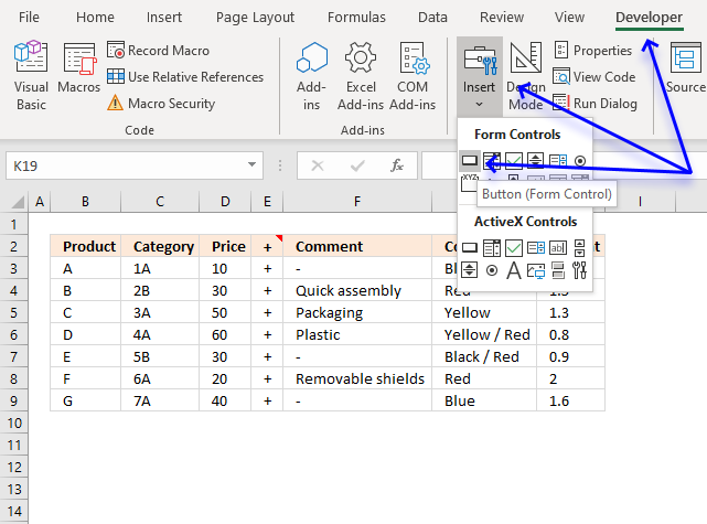
- Press with left mouse button on the "Developer" tab on the ribbon. Search the internet for "Show Developer tab" and your Excel version if it is missing.
- Press with left mouse button on "Insert" button on the "Developer" tab.
- Press with left mouse button on the button in the Form Controls group.
- Move the mouse cursor where you want to place the button on the worksheet.
- Press and hold with left mouse button.
- Drag with mouse to build a button. Don't worry, you can change the size and location later.
- Release left mouse button.
- A dialog box appears.
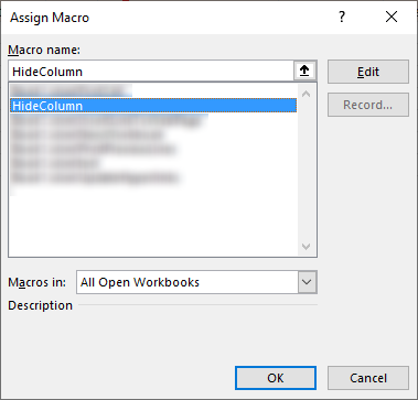
- Press with left mouse button on the macro name, in this case, HideColumn.
- Press with left mouse button on OK button to dissmiss the dialog box.
Press with right mouse button on on the button, a pop-up menu appears. Press with left mouse button on "Assign Macro...". The dialog box shows up again asking for a macro.
3.8 How to hide a row with a button
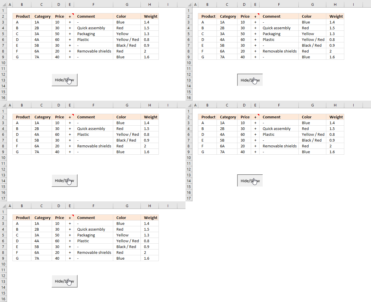

The example demonstrates a button that hides a specific row, press with left mouse button on the button with the left mouse button and it will be hidden if the current state is visible and vice versa.
The animated image above shows a macro that hides entire row 5 when the user press with left mouse button ons on the button named "Hide/Show". The macro toggles row 5 between visible and hidden based on the current condition.
3.9VBA Code
'Name macro
Sub HideRow()

'Check if row 5 is hidden
If Range("5:5").EntireRow.Hidden = True Then

    'Show row 5
    Range("5:5").EntireRow.Hidden = False

'Continue here if row 5 is visible
Else

    'Hide row 5
    Range("5:5").EntireRow.Hidden = True
End If

End Sub
The following VBA macro hides multiple rows, in this example row 5 and 7 are hidden.
'Name macro
Sub HideMultipleRows()

'Save two strings to array variable rW
rW = Array("5:5", "7:7")

'Iterate through values in array variable rW
For Each r In rW

'Check if row is hidden based on value in variable r
If Range(r).EntireRow.Hidden = True Then

    'Show row based on variable r
    Range(r).EntireRow.Hidden = False

'Continue here if row is visible
Else

    'Hide row
    Range(r).EntireRow.Hidden = True
End If

'Continue with next value in array
Next r

End Sub
How to link macro to the button?
4. Hide specific columns programmatically
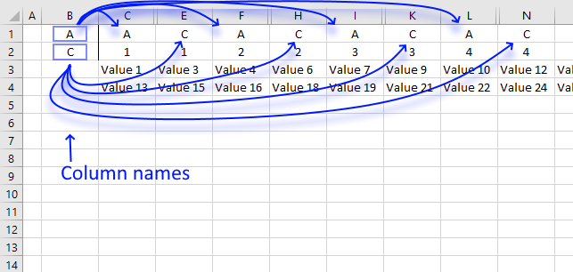
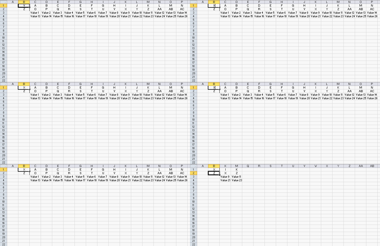
This article describes a macro that hides specific columns automatically based on values in two given cells.
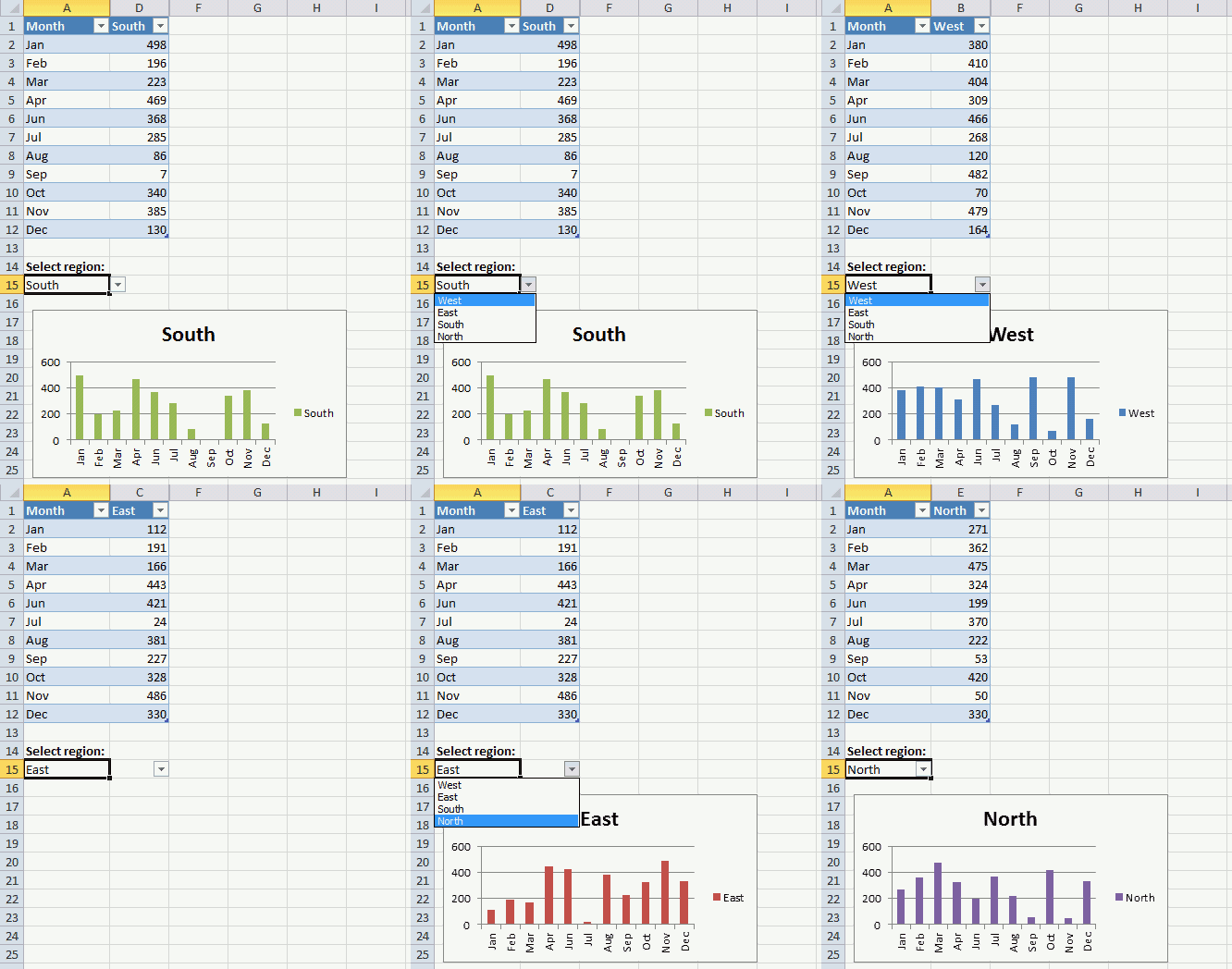
I am also going to show you how to hide columns in an Excel Table programmatically. The Excel Table is the data source for a chart, it changes based on which value the user selects using a drop-down list.
eg:
B1 and B2 hold header names chosen by the user.
range C1 to P2 holds all headers.
Hide ALL columns except those sharing names found in B1 and B2?
4.1 VBA code
'Event code is rund when a cell changes
Private Sub Worksheet_Change(ByVal Target As Range)

'Dimension variables and declare data types
Dim Value As Range, Cells As Range, Cell As Variant
Dim c As Integer, b As Boolean

'Check if cell B1 or B2 is changed
If Not Intersect(Target, Range("B1:B2")) Is Nothing Then

    'Stop screen from refreshing
    Application.ScreenUpdating = False

    'Unhide columns in cell range C:P
    Worksheets("Cyril").Range("C1:P2").EntireColumn.Hidden = False

    'Iterate through 0 (zero) to 13
    For c = 0 To 13

        'Save range object reference to variable Cells
        Set Cells = Worksheets("Cyril").Range("C1:C2").Offset(0, c)

        'Save False to variable b
        b = False

        'Iterate through each cell in variable Cells
        For Each Cell In Cells

            'Iterate through each value in cell range B1:B2 in worksheet Cyril
            For Each Value In Worksheets("Cyril").Range("B1:B2")

                'If statement checks whether variable Value equals variable Cell
                If Value = Cell Then

                    'Save True to variable b
                    b = True
                End If

            'Continue with next value in variable Value
            Next Value

        'Continue with next cell
        Next Cell

        'Check if variable b is equal to False
        If b = False Then

            'Hide column
            Cells.EntireColumn.Hidden = True
        End If

    'Continue with next number
    Next c

    'Show changes to Excel user
    Application.ScreenUpdating = True
End If
End Sub
4.2 Animated image
The animated image above shows what happens when the user enters column header names in cell B1 and B2.
4.3 Where to put the code?
- Press with right mouse button on on the tab with sheet name "Cyril" located at the bottom of your screen.
- Press with left mouse button on on "View Code", this opens the Visual Basic Editor and takes you to the worksheet module.
- Paste VBA code to worksheet module.
- Return to Excel.
5. Hiding columns in a table
The image above shows a drop-down list in cell A15 that allows you to control which data series you want to be graphed. When the value in cell A15 changes the following event macro hides all columns in the Excel Table except the chosen name. The chart changes as well and shows only what the Excel Table shows.
I highly recommend you use a slicer if you have Excel 2010 or a later version, there is no need for a macro.
'Event code is rund when a cell is changed
Private Sub Worksheet_Change(ByVal Target As Range)

'Dimension variable and declare data type
Dim c As Integer

'Check if cell A15 is changed
If Not Intersect(Target, Range("A15")) Is Nothing Then

    'Stop screen from refreshing
    Application.ScreenUpdating = False

    'Unhide all columns for table Table1
    Range("Table1").EntireColumn.Hidden = False

    'Iterate from 2 to the number of columns in Table1
    For c = 2 To Range("Table1").Columns.Count

        'Check if a cell is not equal to the value in cell A15
        If Range("Table1[#All]").Cells(c) <> Range("A15") Then

            'Hide column based on variable c representing the cell number in Table1
            Range("Table1").Cells(c).EntireColumn.Hidden = True
        End If

    'Continue with next number in variable c
    Next c

    'Show changes to user
    Application.ScreenUpdating = True

End If
End Sub
Macro category
Table of Contents Add values to a regular drop-down list programmatically How to insert a regular drop-down list Add values […]
Working with multiple Excel workbooks can be time-consuming, especially when dealing with large datasets spread across multiple files. Fortunately, VBA […]
This article describes how to create a button and place it on an Excel worksheet, then assign a macro to […]
Excel categories
31 Responses to “Auto resize columns as you type”
Leave a Reply
How to comment
How to add a formula to your comment
<code>Insert your formula here.</code>
Convert less than and larger than signs
Use html character entities instead of less than and larger than signs.
< becomes < and > becomes >
How to add VBA code to your comment
[vb 1="vbnet" language=","]
Put your VBA code here.
[/vb]
How to add a picture to your comment:
Upload picture to postimage.org or imgur
Paste image link to your comment.


Oscar,
what code would you suggest in order to allow column resizing in a protected worksheet?
whereas some cells are locked.
would still the vba encounter a Run-time error '424' if a line was added to "bypass" the protection?
(un protect, modify,re-protect)
such as:
Sheets(“Sheet1″).Unprotect Password:=” whatever ”
PROCEDURE
Sheets(“Sheet1).Protect Password:=” whatever “
with the risk of having the sheet unprotected if the procedure fails...
or something like
Private Sub Workbook_Open()
Sheets (" sheetname ") .protect _
Password:=" whatever", _
UserInterfaceOnly:=True
End Sub
Thanks.
Oops,
forgot to add,
would this be included in the first code or should it be a separate code?
Cyril,
You can select "Format rows" and "Format columns" when you protect a sheet.
Now you can use the macro in a protected sheet.
Yes... true.
although I locked the sheet to limit the width... I have many users and some tend to be "artistic" and revamp the files.
Thanks for the reminder.
Cyril,
Try this code:
Private Sub Workbook_SheetChange(ByVal Sh As Object, ByVal Target As Range) Application.ScreenUpdating = False Worksheets(Sh.Name).Unprotect Password:="whatever" On Error Resume Next For Each Value In Target.Columns Worksheets(Sh.Name).Columns(Value.Column).AutoFit Next Value On Error GoTo 0 Worksheets(Sh.Name).Protect Password:="whatever" Application.ScreenUpdating = True End SubThanks Oscar!
Thanks.
One complication:
Given the following setup:
A B C A B C A B C
1 1 1 2 2 2 3 3 3
DATA DATA DATA DATA DATA DATA DATA DATA DATA
DATA DATA DATA DATA DATA DATA DATA DATA DATA
That is the first Header Row contains 3 choices, A or B or C
Then the second Header Row contains as well 3 choices 1 or 2 or 3.
Selecting A would display A1 A2 and A3
Selecting 1 would display A1, B1 and C1
Selecting A and 1 would display A1 only
Selecting none that is leaving the cells B1 and B2 blank would display the whole range
Cyril,
Private Sub Worksheet_Change(ByVal Target As Range) Dim Value As Range, Cells As Range, Cell As Variant Dim c As Integer, b As Boolean If Not Intersect(Target, Range("B1:B2")) Is Nothing Then If Range("B1") = "" And Range("B2") = "" Then Worksheets("Cyril").Range("C1:P2").EntireColumn.Hidden = False Else Worksheets("Cyril").Range("C1:P2").EntireColumn.Hidden = False For c = 0 To 13 Set Cells = Worksheets("Cyril").Range("C1:C2").Offset(0, c) b = False For Each Cell In Cells For Each Value In Worksheets("Cyril").Range("B1:B2") If Value <> "" Then If Value = Cell Then If b = True Then Worksheets("Cyril").Range("C1:P2").EntireColumn.Hidden = True Cells.EntireColumn.Hidden = False Exit Sub End If b = True End If End If Next Value Next Cell If b = False Then Cells.EntireColumn.Hidden = True End If Next c End If End If End SubYes, very nice.
works fine on a mac as well.
added button to execute "unhide".
Here is another way to write the Change event code for the Table (it eliminates iterating the columns)...
Private Sub Worksheet_Change(ByVal Target As Range) If Not Intersect(Target, Range("A15")) Is Nothing Then Application.ScreenUpdating = False With ActiveSheet.ListObjects("Table1") .DataBodyRange.Cells(1).Offset(, 1).Resize(, .DataBodyRange. _ Columns.Count - 1).EntireColumn.Hidden = True .DataBodyRange.Columns(.ListColumns(Range("A15").Value).Index).Hidden = False End With Application.ScreenUpdating = True End If End SubRick Rothstein (MVP - Excel),
Thank you for your contribution!
Could this work for rows? I have a column I need to stay the same size but I need the rows to be re-sized as the user types. Can you help?
Yogi,
Yes!
Private Sub Workbook_SheetChange(ByVal Sh As Object, ByVal Target As Range)

Application.ScreenUpdating = False

For Each Value In Target.Columns
    Worksheets(Sh.Name).Rows(Value.Column).AutoFit
Next Value

Application.ScreenUpdating = True

End Sub
Get the Excel *.xlsm file
Auto-resize-rows.xlsm
Since the code is a toggle, you can eliminate the If..Then..Else..EndIf block and just use a logical expression instead...
Private Sub Worksheet_SelectionChange(ByVal Target As Range) If Not Intersect(Target, Range("D:D")) Is Nothing And Target.Cells.CountLarge = 1 Then Range("E:E").EntireColumn.Hidden = Not Range("E:E").EntireColumn.Hidden End If End SubRick Rothstein (MVP - Excel),
Great, thank you for commenting!
Why is not useful code on Office 2003
Hi! How can I make it work for selected worksheets rather than whole workbook? I need to have one or two worksheets where the column width is set manually. Many thanks for your help in advance.
Justine,
1. Press with right mouse button on a sheet name
2. Press with left mouse button on "View Code.."
3. Copy / Paste the code below
4. Return to excel (Alt + Q)
Private Sub Worksheet_Change(ByVal Target As Range) Application.ScreenUpdating = False For Each Value In Target.Columns Columns(Value.Column).AutoFit Next Value Application.ScreenUpdating = True End SubThank you so much, this is very helpful. I have two worksheets where I already have a code for automatic sorting, and when I paste this second code to the editor then try to add new data I get an error message - Compile error: Ambiguous name detected: Worksheet_Change. Any idea what am I doing wrong? I'll be most grateful for your help.
Justine,
It seems like you have two Worksheet_Change subroutines. You can only have one.
This is great. What change needs to be done in order for it to work with dynamic data (like data populated with index match or vlookup or lookup and contat formula you have). I have my version from your replies as below. Instead of change I thought triggering event with Calculate would work, but it did not.
Also we have about 2000 rows loading dynamically and do not want to overload excel. Thanks a lot in advance.
Private Sub Worksheet_Calculate(ByVal Target As Range)
Application.ScreenUpdating = False
Worksheets(Sh.Name).Unprotect Password:="Password"
On Error Resume Next
For Each Value In Target.Columns
Worksheets(Sh.Name).Rows(Value.Column).AutoFit
Next Value
On Error GoTo 0
Worksheets(Sh.Name).Protect Password:="Password"
Application.ScreenUpdating = True
End Sub
I meant "Lookup_concat" user formula that you mentioned in other tutorial.
Why am I getting "variable not defined" error on first line of the code?
Andrew,
Did you put the code in the workbook module?
Oscar,
This works perfectly for resizing the columns, so thanks for that! I just noticed, though, that the sheet no longer allows for an 'Undo'. Ctrl-Z just gives me a noise indicating that I did something wrong, and the 'Undo' arrow is grayed out. Is there something I can do to fix that? FYI, I'm using Excel 2013.
Thanks,
Zach
Zach
Short answer:
No, that is a disadvantage with the macro.
Long answer:
https://stackoverflow.com/questions/24185942/save-undo-stack-during-macro-run
https://www.jkp-ads.com/Articles/UndoWithVBA00.asp
Hello,
How could I have multiple sets of columns in one sheet that have the show/hide functionality?
Nevermind... I figured out I can just do multiple IF statements in the same Sub.
Thanks for your support Oscar.
In case i Want to apply this formula but to just specific columns... what do I have to change or add on this vba code:
Private Sub Workbook_SheetChange(ByVal Sh As Object, ByVal Target As Range)
Application.ScreenUpdating = False
For Each Value In Target.Columns
Worksheets(Sh.Name).Rows(Value.Column).AutoFit
Next Value
Application.ScreenUpdating = True
End Sub
So far this works great for me, but how do you also have it adjust the height as well as the width in the VBA? So far it just the width. I have sheet with several columns and cells that auto fill from what is selected in the drop down list.