Lookup a date in date ranges and get the corresponding value

This article explains how to search for a specific date and identify a date range in which it falls between the start and end dates. The image above shows a formula in cell C9 that uses the date specified in cell C8 to match a date range.
A date range is matched if the date is larger or equal to the start date and smaller or equal to the end date. The date ranges are in cell range C3:D6.
The date in cell C8 matches date range 4-1-2022 / 6-30-2022, the formula returns a value on the same row from cell range B3:B6, in this case, Item "B".
Table of contents
- Match a date when a date range is entered in a single cell
- Match a date when the start of a new date range is the end of the earlier one
- Find a date within date ranges and return adjacent value - Excel 365
- Use VLOOKUP to search date in date ranges and return value on the same row
- Match a date when date ranges sometimes overlap and return multiple results
1. Match a date when a date range is entered in a single cell
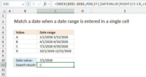
The image above shows a dataset in cell range B4:C8, the first column name is "Value" and the second column is named "Date range". It has text values "A" to "D" in cells B5:B8 and date ranges in cells C5:C8. Column C contains the start and end date separated by a - (hyphen). The formula in cell C11 splits the dates and checks if the given date in cell C10 is in a date range. If true then it returns the adjacent value on the same row from cells B5:B8.
Array formula in C9:
For example, the given date 7/1/2028 is in cell C10. It matches only date range 7/1/2028-9/30/2028, the corresponding value on the same row from cell B5:B8 is value "C".
How to create an array formula
Excel 365 subscribers can skip the following steps describing how to enter an array formula. Excel 365 uses dynamic array formulas which spills values automatically to adjacent cells. They are entered as regular formulas simply by pressing Enter.
- Select cell C9.
- Press with left mouse button on in the formula bar.
- Copy and paste array formula to the formula bar.
- Press and hold CTRL + SHIFT simultaneously.
- Press Enter.
- Release all keys.
1.3 Explaining formula
Step 1 - Calculate character position of hyphen
The FIND function returns the position of a specific string in another string, reading left to right. Note, the FIND function is case-sensitive.
FIND(find_text,within_text, [start_num])
FIND("-", C3:C6)
returns {11; 11; 11; 11}.
Step 2 - Calculate the number of characters in each cell
The LEN function returns the number of characters in a cell value.
LEN(text)
LEN(C3:C6)
returns {21; 21; 21; 21}.
Step 3 - Calculate position from last character
The minus character lets you perform an arithmetic operation, it subtracts one value with another value.
LEN(C3:C6)-FIND("-", C3:C6)
returns {10; 10; 10; 10}.
Step 4 - Extract characters
The RIGHT function extracts a specific number of characters always starting from the right.
RIGHT(text,[num_chars])
RIGHT(C3:C6, LEN(C3:C6)-FIND("-", C3:C6))
returns
{"3/31/2028"; "6/30/2028"; "9/30/2028"; "12/31/2028"}
Step 5 - Convert text to date
The DATEVALUE function returns an Excel date value (serial number) based on a date stored as text.
DATEVALUE(date_text)
DATEVALUE(RIGHT(C3:C6, LEN(C3:C6)-FIND("-", C3:C6)))
returns {39903; 39994; 40086; 40178}.
Step 6 - Check if larger than or equal to
The larger than and equal signs are logical operators, they are used in this example to check if a date is in a date range.
The output is a boolean value TRUE or FALSE, the position of each value in the array correspond to the date ranges.
DATEVALUE(RIGHT(C3:C6, LEN(C3:C6)-FIND("-", C3:C6)))>=C8
returns
{TRUE; TRUE; TRUE; FALSE}.
Step 7 - Check date against end dates
DATEVALUE(RIGHT(C3:C6, LEN(C3:C6)-FIND("-", C3:C6)))>=C8
returns
{FALSE; FALSE; TRUE; TRUE}.
Step 8 - Create number sequence
The ROW function calculates the row number of a cell reference.
ROW(reference)
ROW($C$3:$C$6)
returns
{3; 4; 5; 6}.
Step 9 - Create a number sequence from 1 to n
The MATCH function returns the relative position of an item in an array or cell reference that matches a specified value in a specific order.
MATCH(lookup_value, lookup_array, [match_type])
MATCH(ROW($C$3:$C$6), ROW($C$3:$C$6))
returns
{1; 2; 3; 4}.
Step 10 - Multiply arrays
The asterisk charcater lets you multiply arrays.
(DATEVALUE(LEFT(C3:C6, FIND("-", C3:C6)-1))<=C8)*(DATEVALUE(RIGHT(C3:C6, LEN(C3:C6)-FIND("-", C3:C6)))>=C8), ROW(C3:C6)-MIN(ROW(C3:C6))+1)
returns
{0; 0; 3; 0}.
Step 11 - Sum numbers
The SUMPRODUCT function calculates the product of corresponding values and then returns the sum of each multiplication.
SUMPRODUCT((DATEVALUE(LEFT(C3:C6, FIND("-", C3:C6)-1))<=C8)*(DATEVALUE(RIGHT(C3:C6, LEN(C3:C6)-FIND("-", C3:C6)))>=C8), ROW(C3:C6)-MIN(ROW(C3:C6))+1))
returns 3.
Step 12 - Get value
The INDEX function returns a value from a cell range, you specify which value based on a row and column number.
INDEX(array, [row_num], [column_num])
INDEX($B$3:$B$6, SUMPRODUCT(DATEVALUE(RIGHT(C3:C6, LEN(C3:C6)-FIND("-", C3:C6)))>=C8)*(DATEVALUE(LEFT(C3:C6, FIND("-", C3:C6)-1))<=C8), MATCH(ROW($C$3:$C$6), ROW($C$3:$C$6))))
becomes
INDEX($B$3:$B$6, 3)
and returns "C" in cell C9.
1.4 Get the Excel *.xlsx File
matching-a-date-in-a-date-range v3.xlsx
(Excel 2007- Workbook *.xlsx)
2. Find a date in date ranges and get adjacent value - sorted date ranges
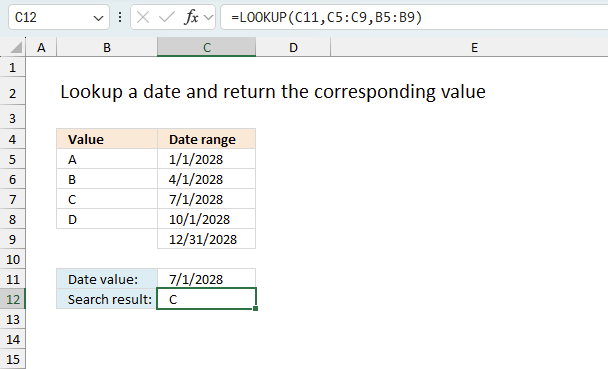
The image above shows a data set, in cell range B4:C9, containing two columns named "Value", and "Date range". There are no gaps between these date ranges which makes it is possible to only use the dates specified in column C. In other words, the end date of the first date range is also the start date of the second date range. This applies to all date ranges.
Formula in cell C9:
Note, there are no gaps between date ranges. If you have gaps use the formula described in section 2.3 or 3.
2.2 Explaining formula
Step 1 - LOOKUP function
The LOOKUP function lets you find a value in a cell range and return a corresponding value on the same row.
LOOKUP(lookup_value, lookup_vector, [result_vector])
The values in lookup_vector must be sorted in ascending order or from A to Z.
Step 2 - Populate arguments
LOOKUP(C8,C3:C6,B3:B6)
lookup_value - The lookup value is in cell C9.
lookup_vector - The lookup cell range is C3:C6. Note start dates are sorted in ascending order.
[result_vector] - The function returns a value from this range on the same row as the matching lookup value.
Step 3 - Evaluate LOOKUP function
LOOKUP(C8,C3:C6,B3:B6)
becomes
LOOKUP(39994, {39814; 39904; 39995; 40087}, {"A"; "B"; "C"; "D"})
and returns "C".
2.3 Lookup with gaps between date ranges - sorted date ranges
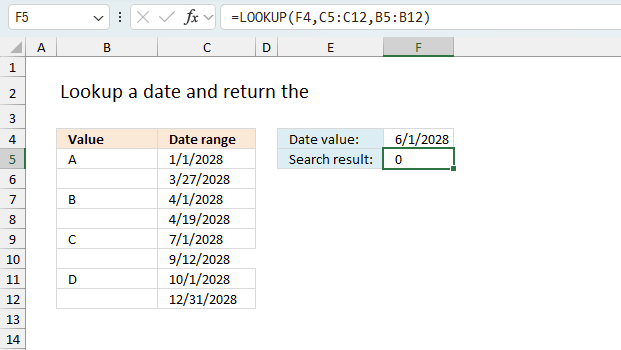
The image above shows how to arrange dates if the date range has a start and end date that doesn't align with the next date range.
For example, date 6/1 in cell F4 is not in any date range, however, it matches the dates between 4/19 and 7/1. The corresponding cell in column B is B8 which is empty indicating this doesn't fall between the date ranges.
This works also if some date ranges align and some don't. Here is an example of that:
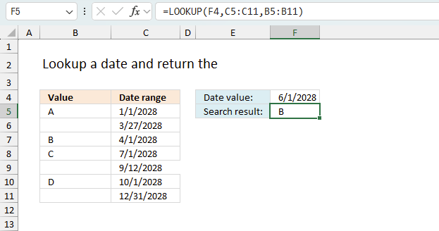
Date range 4/1 - 7/1 has the same end date as the start date in 7/1 - 9/12. The remaining date ranges are not aligned.
3. Find a date within date ranges and return adjacent value - Excel 365
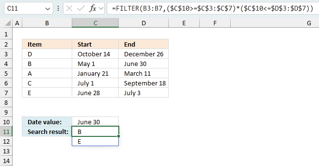
The image above shows an Excel 365 formula that extracts corresponding values from column B if the given date in cell C10 falls between specified start and end date ranges. This works also if multiple date ranges match the given date as shown in this example. This formula works with date ranges in random order meaning they don't have to be sorted in contrast to the formula in section 2 above.
Formula in cell C11:
For example, date "June 30" matches two date ranges "May 1 - June 30" and "June 28 - July 3". The corresponding values on the same rows are "B", and "E".
An Excel 365 dynamic array formula spills values to adjacent cells if needed. This is the case in this scenario shown in the image above. The formula is entered in cell C11 and spills to the cell below. A #SPILL! error is displayed if the destination cells are not empty, in other words, the destination cells are populated with values.
3.2 Explaining formula in cell C9
Step 1 - Check if the end dates is larger or equal to date
The less than, larger than, and equal signs are all logical operators. Logical expressions in Excel are formulas that evaluate to either TRUE or FALSE based on specified conditions. They typically involve logical operators such as =, <, >, <=, >=, and <> to compare values. Logical expressions are fundamental for decision-making functions like IF, AND, OR, and NOT, allowing users to automate actions based on whether a condition is met. These expressions help in filtering data, validating inputs, and performing conditional calculations in spreadsheets.
$C$8>=$C$3:$C$6
returns
{FALSE;TRUE;TRUE;FALSE;TRUE}
Boolean values in Excel are TRUE and FALSE representing the two possible outcomes of a logical evaluation. These values are the result of logical expressions and are used in functions that perform conditional operations. Boolean values can be used in formulas, comparisons, and decision-making functions to control workflow and automate tasks. They are treated as numeric values, where TRUE is equivalent to 1 and FALSE is equivalent to 0, allowing them to be used in calculations and logical operations.
Step 2 - Check if the start dates is smaller or equal to date
$C$8<=$D$3:$D$6
returns {FALSE; TRUE; TRUE; TRUE}.
Step 3 - Multiply arrays - AND logic
The parentheses let you control the order of calculation. The asterisk multiples two numbers or two arrays.
($C$8>=$C$3:$C$6)*($C$8<=$D$3:$D$6)
returns {0;1;0;0;1}
Step 4 - Extract values based on logical expressions
The FILTER function extracts values/rows based on a condition or criteria.
Function syntax: FILTER(array, include, [if_empty])
FILTER(B3:B7,($C$10>=$C$3:$C$7)*($C$10<=$D$3:$D$7))
becomes
FILTER({"D";"B";"A";"C";"E"}, {0;1;0;0;1})
and returns {"B", "E"}.
matching-a-date-in-a-date-range v5
4. Use VLOOKUP to search date in date ranges and return value on the same row
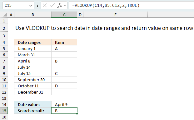
The following formula uses only the VLOOKUP function, however, the dates must be sorted in ascending order and if a date is outside a date ranges 0 (zero) is returned. There can't be any overlapping date ranges and the formula can only return one value.
The example demonstrated in the image above has date ranges in only one column. Every other date is the end date of each date range.
You are also required to have the lookup column in the first column in the cell reference you use in the VLOOKUP function. Example, the second argument in the VLOOKUP function below is this cell reference: B3:C10. The lookup column must be in column B.
Formula in cell C13:
Section 2 describes the LOOKUP function which allows you to specify the lookup_column and the result_column. This is an easier approach than the VLOOKUP function, however, both alternatives requires you to make sure to sort the lookup column from small to large before you use the formula.
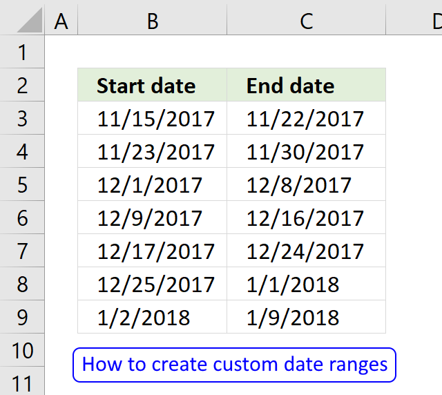
You need to change your date ranges accordingly if you want to use the VLOOKUP function for date ranges entered vertically. However, the VLOOKUP function works perfectly fine if you have date ranges with no gaps between the end dates and start dates, see picture below. You then only need to use the start dates for each date range, example demonstrated in column C see picture below.
4.1 Explaining the formula
Step 1 - VLOOKUP function
The VLOOKUP function lets you search the leftmost column for a value and return another value on the same row in a column you specify.
VLOOKUP(lookup_value, table_array, col_index_num, [range_lookup])
The values in lookup_vector must be sorted in ascending order or from smallest to largest
Step 2 - Populate arguments
VLOOKUP(C12, B3:C10, 2, TRUE)
lookup_value - Date value specified in cell C12
table_array - A cell range containing both the lookup column and the return value column,in this case, B3:C10.
col_index_num - From which column to return a value from.
[range_lookup] - True or False (boolean value). True - approximate match, the leftmost column must be sorted in ascending order, or from small to large. False - Exact match.
Step 3 - Evaluate VLOOKUP function
VLOOKUP(C12, B3:C10, 2, TRUE)
returns "B" in cell C13.
4.2 Get Excel file, see sheet Ex 4
matching-a-date-in-a-date-range v3.xlsx
(Excel 2007- Workbook *.xlsx)
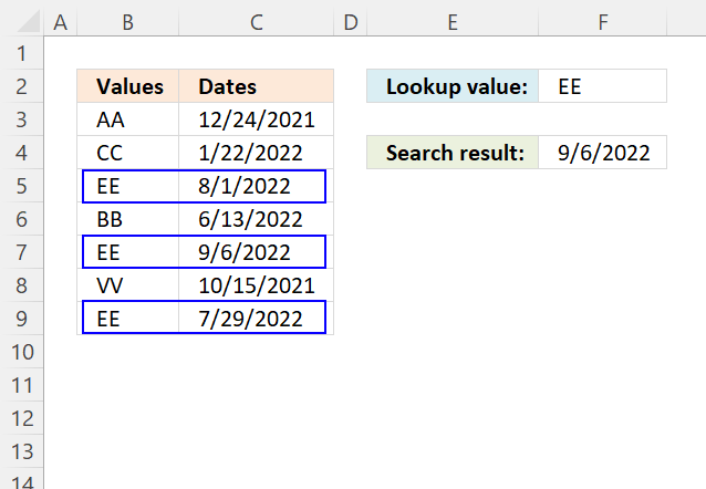
5. Match a date when date ranges sometimes overlap and return multiple results
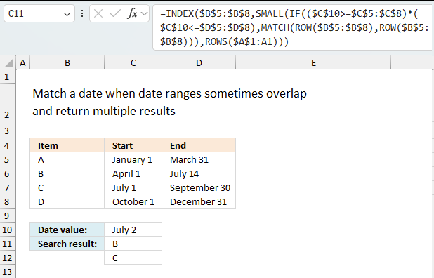
This example demonstrates a formula that returns multiple values if a date condition is met in multiple date ranges. This is only possible if the date overlaps multiple date ranges.
Array formula in cell C9:
For example, date 7/2 above matches both date ranges 4/1 - 14/7 and 7/1 - 9/30. The corresponding values to those date ranges are "B" and "C".
How to copy an array formula
- Select cell C9.
- Copy cell (not formula). (shortcut keys CTRL + c)
- Select cell range C10:C11.
- Paste (shortcut keys CTRL + v).
5.1 Explaining formula
Step 1 - Check if the end dates are larger or equal to the date condition
The less than, larger than, and equal signs are all logical operators. They return a boolean value True or False.
The following expression is the first logical test to check which date range a date matches.
$C$8>=$C$3:$C$6
returns {TRUE; TRUE; TRUE; FALSE}.
Step 2 - Check if the start dates are smaller or equal to the date condition
$C$8<=$D$3:$D$6
returns {FALSE; TRUE; TRUE; TRUE}.
Step 3 - Multiply arrays - AND logic
The parentheses let you control the order of calculation. The asterisk multiples two numbers or two arrays.
TRUE * TRUE = TRUE (1)
TRUE * FALSE = FALSE (0)
FALSE * TRUE = FALSE (0)
FALSE * FALSE = FALSE (0)
The numerical eqivalents to TRUE is 1 and FALSE is 0 (zero)
($C$8>=$C$3:$C$6)*($C$8<=$D$3:$D$6)
returns {0; 1; 1; 0}.
Step 4 - Create a number sequence based on rows in the cell reference
The ROW function calculates the row number of a cell reference.
ROW(reference)
ROW($B$3:$B$6)
returns {3; 4; 5; 6}.
Step 5 - Create number sequence from 1 to n
The MATCH function returns the relative position of an item in an array or cell reference that matches a specified value in a specific order.
MATCH(lookup_value, lookup_array, [match_type])
MATCH(ROW($B$3:$B$6), ROW($B$3:$B$6))
returns {1; 2; 3; 4}
Step 6 - Filter row numbers based on critera
The IF function returns one value if the logical test is TRUE and another value if the logical test is FALSE.
IF(logical_test, [value_if_true], [value_if_false])
IF(($C$8>=$C$3:$C$6)*($C$8<=$D$3:$D$6), MATCH(ROW($B$3:$B$6), ROW($B$3:$B$6)))
returns {FALSE; 2; 3; FALSE}.
Step 7 - Extract k-th smallest row number
The SMALL function returns the k-th smallest value from a group of numbers.
SMALL(array, k)
SMALL(IF(($C$8>=$C$3:$C$6)*($C$8<=$D$3:$D$6), MATCH(ROW($B$3:$B$6), ROW($B$3:$B$6))), ROW(A1))
returns 2.
Step 8 - Get value from cell range
The INDEX function returns a value from a cell range, you specify which value based on a row and column number.
INDEX(array, [row_num], [column_num])
INDEX($B$3:$B$6, SMALL(IF(($C$8>=$C$3:$C$6)*($C$8<=$D$3:$D$6), MATCH(ROW($B$3:$B$6), ROW($B$3:$B$6))), ROW(A1)))
returns "B".
5.2 Get excel file, see sheet Ex 3
matching-a-date-in-a-date-range v3.xlsx
(Excel 2007- Workbook *.xlsx)
Dates category
Question: I am trying to create an excel spreadsheet that has a date range. Example: Cell A1 1/4/2009-1/10/2009 Cell B1 […]
This article demonstrates how to return the latest date based on a condition using formulas or a Pivot Table. The […]
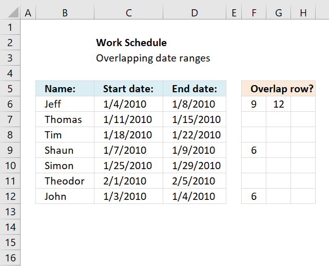
This article demonstrates a formula that points out row numbers of records that overlap the current record based on a […]
Dates basic formulas category
Question: I am trying to create an excel spreadsheet that has a date range. Example: Cell A1 1/4/2009-1/10/2009 Cell B1 […]
This article demonstrates how to return the latest date based on a condition using formulas or a Pivot Table. The […]
Excel categories
57 Responses to “Lookup a date in date ranges and get the corresponding value”
Leave a Reply
How to comment
How to add a formula to your comment
<code>Insert your formula here.</code>
Convert less than and larger than signs
Use html character entities instead of less than and larger than signs.
< becomes < and > becomes >
How to add VBA code to your comment
[vb 1="vbnet" language=","]
Put your VBA code here.
[/vb]
How to add a picture to your comment:
Upload picture to postimage.org or imgur
Paste image link to your comment.
This much shorter formula appears to work also...
=LOOKUP(C8,RIGHT(C$3:C$6,10)-91+(C8=--(YEAR(C8)&"-03-31")),B$3:B$6)
Very interesting! Thanks!
Hi,
What type of formula could be used if you weren't using a date range and your data was not concatenated?
ie: Input Value 1.78 should return a Value of B as it is between the values in Range1 and Range2
Range1 Range2 Value
1.33 1.66 A
1.67 1.99 B
2.00 2.33 C
MT,
see this post: https://www.get-digital-help.com/return-value-if-in-range-in-excel/
Hi!!
This is Ramki. Require your help to fix my concern.
Need a formula to return multiple values while using a double look up formula (Index/Match).
Hi! my date range is set up in two columns
A B C
Start_Date End_Date Item
1-1-12 2-1-12 Text_1
2-2-12 2-15-12 Text_2
I have another list where dates are in sequence and want to lookup text value for each day
A B
Date Item_result
1-1-12 Text_1
1-2-12 Text_1
Ahmed Ali,
I added new content to this post. See:
Match a date when a date range is entered in two cells
Can't thank you enough will give it a try
Again can't thank you enough it worked like a charm. the only thing is that when i search for a date that does not have a task it returns the last task. how can i avoid that. thanks
Hi,
Regarding the formula for "Match a date when date ranges sometimes overlap and return multiple results", is there a way to revise the formula to just look at the dates and indicate if there is crossover?
For example, if I have start date and end dates in four columns and start date in B1 is 1/1/10 and end date in B2 is 12/31/14 and start date in D2 is 10/1/13 and end date in E2 is 10/31/13, I'd like the formula to recognize that the 10/1/13-10/31/13 date range crosses over within the 1/1/10-12/31/14 date range.
Is this possible?
Thanks!
Brett,
I think this post is what you are looking for:
Find overlapping date ranges in excel
Thanks Oscar!
Oscar,
in 2010 excel this isnt working? im getting a #value! error?
I saved your worksheet and I press with left mouse button on c9 and hit enter and it returns the error, any idea what's going on?
anon,
Create an array formula! Instructions above!
Hi Oscar,
I need a fomula that gives me the number of days contained in a range that overlap anoter range... not sure if that is clear enough...
Rene,
read this post: Days contained in a range that overlap another range
[...] Rene asks: [...]
SIR, I AM TRYING TO FIND THE TOTAL OF QUANTITIES DURING GIVEN DATE RANGE IN EXCEL SHEET. SUPPOSE THE QUANTITIES ON EACH OF THE DAY FROM 1 TO 30 IS GIVEN, I NEED TO FIND SUM OF QUANTITIES DURING 7 TO 13. PLEASE HELP. THANKS. SRINIVAS
srinivas,
Hi! my date range is set up in two columns as ALI has
A B C
Start_Date End_Date Item
1-1-12 2-1-12 Text_1
2-2-12 2-15-12 Text_2
I have another list where dates are in sequence and want to lookup text value for each day
A B
Date Item_result
1-1-12 Text_1
1-2-12 Text_1
but if i copy formula into rows in B columns it dost work. thnx
Jan,
try this array formula:
Dear sir,
how do I use sum if to show for example to extract those quantity that match a date range like from 1.1.12 to 31.12.12
1.1.12 80 qty 80
1.11.11 50 0 (as this does fall within date range)
david,
Did you read my answer to srinivas?
https://www.get-digital-help.com/formula-for-matching-a-date-within-a-date-range-in-excel/#comment-54360
Dear Sir,
I am not sure what I am doing wrong, the following is my data and formula I am using, I initially copy one of your examples and change the value field from A,B,C, ETC to 300,320,340, etc tried diff format (gen, num)added rows and keep getting #VALUE! error, made sure fields have same format as the example but once I added the additional rows I get the error, let me know if you can help.. your help is highly appreciated. Grace
=INDEX($B$3:$B$15,MIN(IF((DATEVALUE(RIGHT(C3:C15,LEN(C3:C15)-FIND("/",C3:C15)))>=C17)*(DATEVALUE(LEFT(C3:C15,FIND("/",C3:C15)-1))<=C17),MATCH(ROW($C$3:$C$15),ROW($C$3:$C$15)),"")))
B C
Value Date range
3 300 2013-07-01/2014-06-30
4 320 2012-07-01/2013-06-30
5 340 2011-07-01/2012-06-30
6 360 2010-07-01/2011-06-30
7 380 2009-07-01/2010-06-30
8 400 2008-07-01/2009-06-30
9 420 2007-07-01/2008-06-30
10 440 2006-07-01/2007-06-30
11 460 2005-07-01/2006-06-30
12 480 2004-07-01/2005-06-30
13 500 2003-07-01/2004-06-30
14 520 2002-07-01/2003-06-30
15 540 2001-07-01/2002-06-30
16
17 Date value: 7/1/2010
18 Search result: #VALUE!
Grace Langford,
You forgot to enter it as an array formula.
Get the Excel *.xlsx file
Grace-Langford.xlsx
Many thanks, Oscar. I'm tired and cross-eyed and your formula saved me a lot of time. Worked beautifully!
Hello Oscar!
My situation is similar, but not identical to your examples:
Sheet 1 provides a date range in two cells:
1.2013 2.2013
2.2013 3.2013...
Sheet 2 provides specific dates and values
3.1.2013 500$
5.2.2013 700$...
What I want to do now is insert the Values from Sheet 2 next to the right date ranges in Sheet 1. Please note that there is only one date (and thus one value) for each date ranch.
1.2013 2.2013 500$
2.2013 3.2013 700$
Usually I would use Vlookup and match the dates, but that doesn't work since I have a date range.
I would be very thankful for your help. This problem seems so easy but I can't seem to figure out a solution!
Thanks and best regards!
Hi Oscar,
Based on the staff's joining date, the excel file should display the Percentage entitlement for that staff
Description Grade %
Joined after 01.07.2013 to 31.12.2014 8 % Nil
Joined between 01.07.2012 and 30.06.2013 8 % 5
Joined between 01.07.2011 and 30.06.2012 8 % 8.33
Joined between 01.07.2010 and 30.06.2011 8 % 16.66
Joined between 01.07.2003 to 01.07.2010 8 % 20
joined between 01.07.2003 to 30.06.2013 7 % 25
Pls. could U assist?
Rgds
Hi Oscar
I am new to your site and to posting.
I am in need of some help.
I have 2 data sets. First data set contains 3 columns of data: 1)vehicle unit#, a driver ID# and the date/time of a transaction.
The problem is that often this dataset has a null value for the tractor#, so I need to find out what tractor this driver had during the time the transaction occurred.
I have a second file obtained from OBC (On-board Computer) data that contains Login times and logout times as well as the driver#, Tractor#,Login Date/Time, Logout Time.
There can be many drivers in file 2 that are logged in with a date range that could include transaction date from file 1, so I need to be able to find not only the date within a range, but specific to the driverID.
IE: File 1
DriverId Tractor# Transaction Date
MORT 02/02/2015 04:34:00
MORT 02/02/2015 18:04:00
MORT 02/02/2015 18:59:00
JOHA 02/02/2015 03:35:00
LITMAR 02/02/2015 03:46:00
RODB 02/02/2015 10:15:00
Sorry - Sent previous post without finishing:
IE: File 1
DriverId Tractor# Transaction Date
MORT 02/02/2015 04:34:00
MORT 02/02/2015 18:04:00
MORT 02/02/2015 18:59:00
JOHA 02/02/2015 03:35:00
LITMAR 02/02/2015 03:46:00
RODB 02/02/2015 10:15:00
IE: File 2
Driver ID Vehicle# Login Date/Time Logout Date/Time
MORT 040 02/02/2015 05:20:09 02/02/2015 15:11:25
JOHA 318 02/02/2015 01:35:00 02/02/2015 05:35:00
LITMAR 5129 02/02/2015 01:46:00 02/02/2015 05:46:00
RODB 5101 02/02/2015 01:15:00 02/02/2015 11:15:00
I have daily temperature data for over 50 stations ranging from 2005-2012. I am looking for a formula that will give me the station Name, date closest 12/31/2012, and the temperature value for that date.
I tried vlookup/match/INDEX lookup up or match station than I am unable to index date
My column A is DATE, column B has letters A-H which can repeat and varies with the dates, columns C and D have integers. I am looking for a formula to be in a cell in column E that can give me the value from either C/D if a cell value in column F (can be letters from A-H) matches with the letter in column B and the date is the MOST RECENT DATE. Thanks to everyone who can help me.
Hi,
can anybody help me solve following problem.
Table1
item no - start date - end date - value
A 01.01.16 21.02.16 10
A 22.02.16 31.12.16 20
B 01.01.16 31.12.16 30
Depending on a specific date within the range, the correct value shall be used in following formula:
item no date value
A 20.02.16 VLOOKUP(item no;Table1;4)- Result 10
B 25.02.16 VLOOKUP(item no;Table1;4)- Result 30
A 25.02.16 VLOOKUP(item no;Table1;4)- Result 20
Hi Oscar,
I have
name1 | division |...other columns...| start date of vacation | end date of vac (but start date and end date of vacation are in more than two columns (they are using more than one part of vacation ex: start | end, start|end...)
i need to extract name1, division, start date, end date for any given date
Thank You
counting people on vacation
Hi,
I have a set date that is a baseline. I can move it 60days either side as a maximum.
Qs. I have 300 rows of data each has its own populated baseline date (say row 1 is 30-6-2016 and row 300 is 25-9-2023) but want to align dates by moving some forward and some back for efficiency.
Do I have to first individually make a start date and end date range on each row from the baseline date or is there a formula that can say -60 days (30-6-2016) +60 days
Hi Oscar,
Could you help me solve this problem. I have sets of data both our date based. i.e, what I have below.
4.1.1990 33234 2.1.1990 2345
5.1.1990 33245 4.1.1990 2356
6.1.1990 33265 5.1.1990 2354
7.1.1990 33678 6.1.1990 2367
7.1.1990 2314
What I am trying to do is match the data from the second set of data to the first set of data so that the date lines up. The extra days in the second data will be disregarded as i don't need them.
I have tried many different types of formulas but till not can't find a solution.Doing this manually takes way to long as some of my data spans 25 years.
If you can help I would be very thankful :-)
Hi Merlin
I would separate the contents of one cell into multiple columns, on both data sets. Text-to-columns allows you to do that.
You find Text-to-columns on tab "Data", on the ribbon.
Use INDEX + MATCH to line the dates up.
Formula in cell C1:
=INDEX(Sheet2!A$1:A$5, MATCH(Sheet1!$A1, Sheet2!$A$1:$A$5, 0))
Copy cell C1 (not formula) and paste it to remaining cells in column C and D.
I have a date range A1(12/06/2016) to B1(20/10/2016) and date of joining(DOJ) in C1(15/07/2000). In D1 I want to return 20 otherwise "" if only the DOJ(D1) 15th July matches the date range regardless of the year.
Note: The date format is in (dd/mm/yyy).
I have searched the web but yet to find an answer of this kind. An answer in IF formula(excel) will be great since I don't understand SQL.
Thanks in advance.
John Sanil
John Sanl
This formula works for me:
Thanks Oscar,
Your formula gave me a good relief which I had been searching the web for a long time.
But Sorry, I think, I misinterpreted the way I put in the query.
D1 works perfectly till 31/12/2016 but has it crosses over to the next year say 01/03/2017 (dd-mm-yyy) the answer shows blank even though date of joining ie. 15th July is within date range 12/06/2016 to 01/03/2017. Is there a possible solution for this?
Thanks in advance for the answer
John
John Sanl
I understand, this formula seems to do the work:
=IF(YEAR(A1)=YEAR(B1), IF((DATE(1900,MONTH(A1), DAY(A1))<=DATE(1900,MONTH(C1), DAY(C1)))*(DATE(1900,MONTH(B1), DAY(B1))>=DATE(1900, MONTH(C1),DAY(C1))),20,""), IF((DATE(1900,MONTH(A1), DAY(A1))>DATE(1900, MONTH(C1),DAY(C1)))*(DATE(1900, MONTH(B1), DAY(B1))
Please help
=IFERROR(INDEX(B$4:B$16;SMALL(IF(($B$24>=$I$4:$I$16)*($B$24=$N$4:$N$16)*($B$24<=$P$4:$P$16);MATCH(ROW($B$4:$B$16);ROW($B$4:$B$16)));ROW(A1)));"")
how can I combine these two ranges into one (actualy i have 4 - I and J, N and P,....)? It needs to work like an OR function
Thank You
=IFERROR(INDEX(B$4:B$16;SMALL(IF(($B$24>=$I$4:$I$16)*($B$24=$N$4:$N$16)*($B$24<=$P$4:$P$16);MATCH(ROW($B$4:$B$16);ROW($B$4:$B$16)));ROW(A1)));"")
getting a value error using formula below:
=INDEX($B$2:$B$77,MIN(IF((DATEVALUE(RIGHT(C2:C77,LEN(C2:C77)-FIND("/",C2:C77)))>=C80)*(DATEVALUE(LEFT(C2:C77,FIND("/",C2:C77)-1))<=C80),MATCH(ROW($C$2:$C$77),ROW($C$2:$C$77)),"")))
tony,
Use "Evaluate Formula" on tab "Formulas" on the ribbon.
That will tell you where the error is.
Great Thanks to you as the solutions provided are terribly simple after days of searching for something similar!
Hi, thanks for the formula. In the case of "Match a date when a date range is entered in two cells"
What is the value if no range is matched? How can the formula return a default value in case it doesn't match any range?
Thanks in advance!
Ray
How to retrieve information from another sheet?
Match name by latest 4 max dates.
Sheet 1 has information
ie ; Column A Name & appears 20 times
; Column B Dates & same date appears 100 times
; Column C Distance
; Last Column is Z
Sheet 3 formula match name with latest 4 dates & across columns to last column Z
; Column A6 references Name ; Formula Column N6 Max Date ; M6
; Formula Column N7 2nd max Date ; O7
; Formula Column N8 3rd max Date ; O8
; Formula Column N9 4th max Date ; O9
Formula eg; =VLOOKUP(A6,'QLD RESULTS'!A:A,1,FALSE)
=VLOOKUP(A6,'QLD RESULTS'!A:B,2,FALSE)
=VLOOKUP(A6,'QLD RESULTS'!A:C,3,FALSE)
Regards
Tony
=INDEX($B$3:$B$6, SMALL(IF(($C$8>=$C$3:$C$6)*($C$8<=$D$3:$D$6), MATCH(ROW($B$3:$B$6), ROW($B$3:$B$6))), ROW(A1)))
What is the meaning of ROW(A1)?
Can you also give step by step break down of this formula? I am having hard time understanding this.
Hi Oscar,
Need your help with figuring out a formula.
I have a sheet 1 with 4 columns and following values:
Date start time End Time Analyst
1/5/2021 1:30 PM 4:00 PM Analyst 1
1/5/2021 4:00 PM 6:30 PM Analyst 2
1/6/2021 6:30 PM 9:00 PM Analyst 3
Sheet 2 contains just 1 column:
DateandTime
1/6/21 7:53 PM
1/7/21 7:03 PM
1/5/21 2:51 PM
I want to find to populate the name of the Analyst in sheet 2 if Dateandtime value matches any of the values in Sheet1. For instance, 1/6/21 7:53 PM this value should give me Analyst3 and 1/5/21 2:51 PM should give me Analyst1.
Please help to find out the formula.
Thanks,
Jasmeet
Hi Oscar
Would you please help with a formula.
I have a historical price table for say item ‘A’ where prices have increased at different times over the last 10 years.
Let’s say Column A shows the date of each price change and Column B the corresponding new price.
How would I write a formula to tell me what the price would have been if I enter a specific date in a cell?
Thanks
Sam
First of all I'd like to thank you for giving me exactly what I needed.
The only problem I'm facing is, when formula can't find a matching date, it shows #NUM! Error.
Here's the code (I removed the end date because I didn't need it)
{=INDEX($B$3:$B$10,SMALL(IF(($C$12=$C$3:$C$10),MATCH(ROW($B$3:$B$10),ROW($B$3:$B$10))),ROW(A1)))}Also here's the screenshot from your Workbook
https://postimg.cc/r0nHcF9M
I tried
{=IF(INDEX($B$3:$B$10,SMALL(IF(($C$12=$C$3:$C$10),MATCH(ROW($B$3:$B$10),ROW($B$3:$B$10))),ROW(A1)))="0","",INDEX($B$3:$B$10,SMALL(IF(($C$12=$C$3:$C$10),MATCH(ROW($B$3:$B$10),ROW($B$3:$B$10))),ROW(A1))))}But no luck. I want to show empty cell if formula returns no results.
Hi Oscar,
Need your help with figuring out a formula.
I have a sheet 1 with 4 columns and following values:
Suppler Name Item Date WEF Rate
Chandu Vegetables Bhindi 01-Jan-23 13.00
Chandu Vegetables Bhindi 10-Jan-23 19.00
Hayat Supplier Bhindi 02-Jan-23 12.00
Hayat Supplier Bhindi 06-Jan-23 14.00
Hayat Supplier Bhindi 08-Jan-23 18.00
Kishore Vegetable Bhindi 08-Jan-23 17.00
Kishore Vegetable Tomato 08-Jan-23 9.3
Shakti Tomato Tomato 01-Jan-23 9.35
Shakti Tomato Tomato 05-Jan-23 9.40
Shakti Tomato Tomato 10-Jan-23 9.50
Super Vegetables Tomato 01-Jan-23 9.00
Super Vegetables Tomato 05-Jan-23 9.25
Super Vegetables Tomato 08-Jan-23 8.00
Super Vegetables Tomato 10-Jan-23 9.65
Vikrant Fruits Bhindi 10-Jan-23 18.50
Sheet 2 Need Rate for following
Suppler Name Item Date WEF Rate?
Super Vegetables Tomato 02-Jan-23
Hayat Supplier Bhindi 04-Jan-23
Chandu Vegetables Bhindi 05-Jan-23
Hayat Supplier Bhindi 07-Jan-23
Kishore Vegetable Tomato 08-Jan-23
Kishore Vegetable Tomato 09-Jan-23
Kishore Vegetable Bhindi 09-Jan-23
Chandu Vegetables Bhindi 10-Jan-23
Vikrant Fruits Bhindi 10-Jan-23
Shakti Tomato Tomato 10-Jan-23
Chandu Vegetables Bhindi 11-Jan-23
Vikrant Fruits Bhindi 11-Jan-23
I want to find to populate the Rate in sheet 2 if Supplier Name, Item Name matches while Date matches or it should take Previous rate .
Please help to find out the formula.
Thanks,
Sohel Ahmed
Sohel Ahmed,
Here is a formula I think you are looking for:
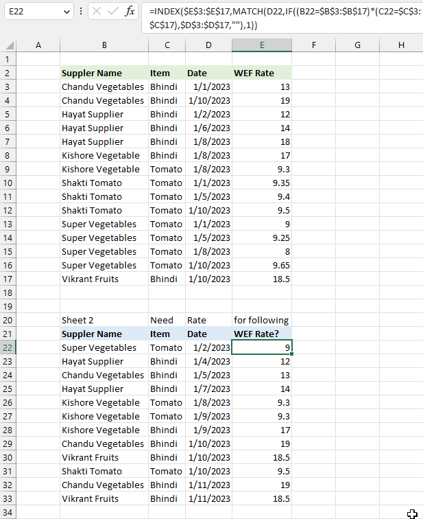
As long as your dates are sorted in ascending order and into groups based on "Supplier Name" and "Item" the above formula will work.
Hi there,
Need a hand with a similar date formula
I have one sheet with 2 columns with the following;
FY & Date Range
2021-2022 01/04/2021 - 31/05/2022
2022-2023 01/04/2022 - 31/05/2023
2023-2023 01/04/2023 - 31/05/2024
I have a date range which I would need the FY.
For example;
I have a date range 05/05/2022-25/12/2022 (this would be FY 2022-2023) is there a formula for this?
Also, if the date range goes over 2 FY what would be the best formula?
for example;
25/02/2023 - 19/06/2023 (FY are 2022-2023 & 2023-2024)
Thanks
Qas,
I created helper columns to keep the formulas as small as possible:
Qas.xlsx