Extract records between two dates
This article presents methods for filtering rows in a dataset based on a start and end date.
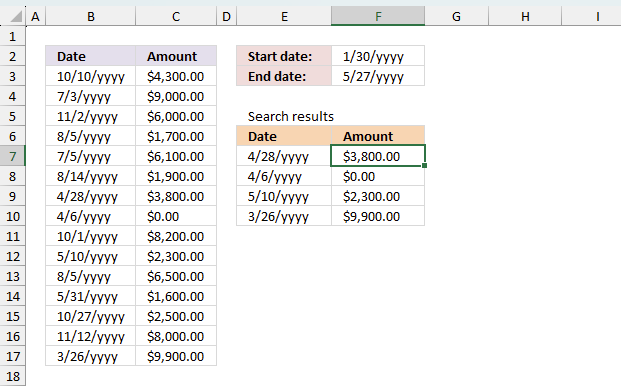
The image above shows a formula in cells E7:F10 that extracts rows from cell range B3:C17 if the dates fall between the conditions specified in cells F2 and F3.
I will be showing you how to filter dates using these Excel features:
- Excel 365 dynamic array formula - more powerful Excel functions.
- Excel formula - earlier Excel versions.
- Excel Table - easy to use.
- Excel Table and VBA.
- Autofilter - easy to use.
- Advanced filter - handles more complicated criteria.
Dynamic array formulas require Excel 365, Excel Tables require Excel 2007 or a later version. The remaining methods should work on almost any Excel version.
What's on this webpage
- Filter rows using array formulas based on a date range - Excel 365
- Filter rows using array formulas based on a date range - earlier Excel versions
- Filter rows using an Excel table based on a date range
- Filter rows using Excel table and VBA based on a date range
- Filter rows based on a date range - Autofilter
- Filter rows based on a date range - Advanced filter
1. Filter rows using array formulas based on a date range - Excel 365
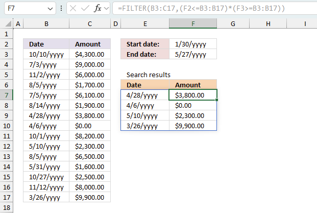
This example shows the new FILTER function in cell E7, it uses the start and end dates to filter rows containing a date that falls between the start and end dates. The result is an array that is returned to cells below and to the right automatically.
Excel 365 dynamic array formula in cell E7:
Dynamic array formulas are a new feature in Excel 365 that allows you to enter a single formula in a cell and get results that automatically spill into other cells, as far as needed. This can save you time and make your formulas more efficient, as you don't need to create separate formulas for each cell or use the more complicated array formulas.
To create a dynamic array formula, you just need to enter the formula in a cell and press Enter. The results will automatically spill into the surrounding cells, as long as those cells are empty. You will get a a #SPILL error if adjacent cells are populated.
The dynamic array formula spills values to cells below or cells to the right depending on the result array size and shape.
Explaining formula
The FILTER function lets you do amazing things that were not possible before, you needed much larger formulas in earlier Excel versions.
Step 1 - Compare dates to the start date
The less than, greater than, and equal signs are logical operators that let you compare values in Excel formulas, in this case, date values. The result is a logical value, in other words, a boolean value TRUE or FALSE.
Date values in Excel are actually stored as whole numbers. January 1, 1900, is the start date and each subsequent day is represented by a higher serial number. For example, January 1, 1900, is represented by the serial number 1, January 2, 1900, is represented by the serial number 2, and so on.
F2<=B3:B17 returns {TRUE; TRUE; TRUE; ... ; TRUE}
Step 2 - Compare dates to the end date
F3>=B3:B17 returns {FALSE; FALSE; FALSE; ... ; TRUE}
Step 3 - Multiply boolean values
Multiplying boolean values results in AND logic being performed, TRUE if all of the conditions are TRUE, and FALSE if any of the conditions are FALSE.
Here are the possible results of multiplying boolean values:
TRUE * TRUE = TRUE
TRUE * FALSE = FALSE
FALSE * TRUE = FALSE
FALSE * FALSE = FALSE
However, keep in mind Excel converts the result to their numerical equivalents:
TRUE - 1
FALSE - 0 (zero)
Also, in this particular example, Excel multiplies values that correspond to its position in the array meaning the first value in the first array is only multiplied by the first value in the second array and so on.
Using parentheses allows you to specify the order in which the operations should be performed. In this case, it is important to compare the values before multiplying them, as not doing so will result in incorrect output.
(F2<=B3:B17)*(F3>=B3:B17) returns {0;0;0;0;0;0;1;1;0;1;0;0;0;0;1}
Step 4 - Filter rows based on logical test
The FILTER function extracts values/rows based on a condition or criteria.
Function syntax: FILTER(array, include, [if_empty])
FILTER(B3:C17,(F2<=B3:B17)*(F3>=B3:B17)) returns {45044,3800; 45022,0; 45056,2300; 45011,9900}
2. Filter rows using array formulas based on a date range - earlier Excel versions
This example demonstrates a formula that works in older Excel versions. It is a larger formula and I recommend Excel 365 subscribers to use the formula in section 1 that is specifically for Excel 365.
The formula is an array formula and must be entered in a particular way. Here is how:
- Copy the formula below.
- Select the destination cell.
- Paste the formula to the destination cell, there are two ways:
- Shortcut: Press and CTRL key and then press v once. Release CTRL key.
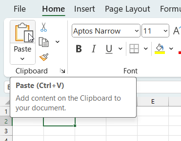
- Use the ribbon: Go to tab "Home" on the ribbon. Press with left mouse button on button "Paste".
- Use the mouse: Press with right mouse button on on the destination cell. A popup menu appears. Press with left mouse button on the "Paste" button on the popup menu.
- Press and hold CTRL and SHIFT keys at the same time.
- Press Enter once.
- Release all keys.
The formula has a leading and trailing curly bracket. Don't enter these characters yourself, they appear automatically.
Array formula in cell E7:
You now need to copy the cell to adjacent cells as far as needed. Here is how:

The animated image above demonstrates how t:
- Copy the formula using the dot on the lower right corner of the cell.
- change the formatting from date to currency using the "Format painter" on the ribbon.
You can also copy/paste using these steps:
- Select the cell containing the formula.
- Copy the cell containing the formula, you have two options:
- Shortcut: Press and hold CTRL key. Press c once. Release CTRL key.
- Use the ribbon: Go to tab "Home" on the ribbon. Press with left mouse button on button "Copy".
- Use mouse: Press with right mouse button on on the cell containing the formula. A popup menu appears. Press with left mouse button on the "Copy" button on the popup menu.
- Paste to the destination cells.
How to change F7:F10 cell formatting:
- Select a cell containing the source formatting, in this example any cell in C3:C17.
- Double-press with left mouse button on the left mouse button on the "Format Painter" button on the ribbon tab "Home".
- Select cell range F7:F10.
See the animated image above.
2.3 How to remove #num errors
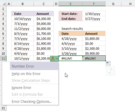
The array formula demonstrated in section 2 above shows an Excel error when no more values can be displayed. The formula returns a #NUM! error that can be hidden using the IFERROR function.
The formula above shows how to combine the IFERROR function and the formula. It returns a blank cell instead of the #NUM! error.
The IFERROR function if the value argument returns an error, the value_if_error argument is used. If the value argument does NOT return an error, the IFERROR function returns the value argument.
Function syntax: IFERROR(value, value_if_error)
2.4 Get the Excel *.xls file
filter-records-between-two-dates.xls
(Excel 97-2003 Workbook *.xls)
3. Filter rows using an Excel table
This example shows how to filter rows in an Excel Table based on a date range. First, we will convert the data set to an Excel Table. Second, we will learn how to filter the data using a start and end date.
Convert a range to an Excel table
- Select cell range A2:B38.
- Go to tab "Insert" on the ribbon.
- Press with left mouse button on "Table" button. A popup menu appears. Enable the check box if the data set has column headers.
- Press with left mouse button on the OK button.
The data set is now an Excel Table which has a lot of benefits:
- Sort data.
- Filter data.
- Change Table styles.
- Create banded rows and/or columns.
- Create a total.
Filter dates in an Excel Table
- Press with left mouse button on the "black arrow" near header name Date.
- Hover over "Date filters" with the mouse pointer. A popup menu appears.
- Press with left mouse button on "Between...". See the image below.
- Select the start date and the end date.
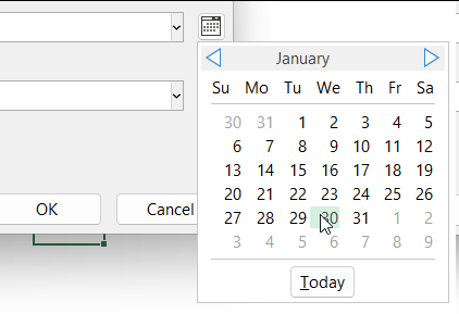
- Press with left mouse button on OK button to apply changes.
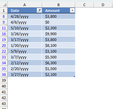
The Excel Table instantly shows the filtered data. The blue row numbers tells you that the Excel Table is filtered as well as the icon on the button next to the column name has changed.
4. Filter rows in an Excel table using VBA

In this example, you can type a start date in cell B1 and an end date in cell B2. Press the button named "Filter" and the Excel Table is instantly filtered. The button is a "Form Control" button that is assigned to a VBA macro.
What is a Form Control?
Form Controls are built-in user interface elements in Microsoft Excel and other Microsoft Office applications that allow users to interact with spreadsheets or documents. These controls include buttons, checkboxes, dropdown lists, scroll bars, and more. Form Controls are relatively simple and are linked directly to spreadsheet cells, allowing for easy data manipulation without the need for complex coding.
- Simple to use and configure.
- Work with Excel’s built-in macros and formulas.
- Do not require programming knowledge (VBA is optional).
- Faster and more lightweight compared to ActiveX controls.
- Limited customization options.
What is VBA?
VBA (Visual Basic for Applications) is a programming language developed by Microsoft that is used for automating tasks in Microsoft Office applications such as Excel, Word, and Access. It allows users to create macros, automate repetitive tasks, and enhance Office functionality with custom scripts.
What is a macro?
In Microsoft Excel, a macro is a sequence of instructions written in Visual Basic for Applications (VBA) that allows you to automate repetitive tasks time consuming tedious tasks. Macros can perform a wide range of actions from simple formatting changes to complex data manipulations.
How to get this to work?
Copy the VBA code below into a regular module. Create a button and assign the macro. There are more detailed instructions below.
4.1 VBA code
Sub TblFilterDates()

Worksheets("Sheet3").ListObjects("Table13").Range.AutoFilter _
Field:=1, _
Criteria1:=">=" & Worksheets("Sheet3").Range("B1") _
, Operator:=xlAnd, _
Criteria2:="<=" & Worksheets("Sheet3").Range("B2")
End Sub
This VBA macro filters a table named "Table13" on a worksheet called "Sheet3" based on dates specified in cells B1 and B2, in the first column (Field:=1) of the table. The filter criteria are :
- Criteria1: ">=" & Worksheets("Sheet3").Range("B1")
This specifies that the dates in the first column of the table should be greater than or equal to the date in cell B1 on the "Sheet3" worksheet. - Criteria2: "<=" & Worksheets("Sheet3").Range("B2")
This specifies that the dates in the first column of the table should be less than or equal to the date in cell B2 on the "Sheet3" worksheet. - Operator:=xlAnd
This specifies that the filter should use "AND" logic to combine the two criteria meaning both criteria must match.
The AutoFilter method is used to apply a filter to a range of cells or a table in a worksheet. When a filter is applied, only the rows that meet the specified criteria are displayed, and the remaining rows are hidden. The AutoFilter method can be used to filter data based on a specific value, a range of values, or a pattern.
4.2 Where to copy VBA code?

- Press Alt+F11 to open the Visual Basic Editor (VBE).
- Press with mouse on Insert.
- Press with mouse on "Module" to insert a new module to you workbook.
- Copy and paste code into code window, see the image above.
4.3 How to create a button (Form Control)

- Press with left mouse button on "Developer" tab on the ribbon.
- Press with left mouse button on "Insert" button.
- Create a button (form control) on the worksheet.
- Press with right mouse button on on the button.

A popup menu appears. Press with left mouse button on "Assign Macro...". - A dialog box shows up.

- Select the macro name.
- Press with left mouse button on OK button.
4.4 Get Excel *.xlsm (macro-enabled) file
filter-records-between-two-dates.xlsm
(Excel 2007 MacroEnabled Workbook *.xlsm)
5. Filter rows based on a date range - Autofilter

This section demonstrates how to filter the data set in columns B and C using a start and end date.
5.1 Create Autofilter
- Select any cell in the data set.

- Go to tab "Data" on the ribbon.
- Press with left mouse button on the "Filter" button.

- The column headers now show a button containing an arrow.

5.2 Apply filter to data
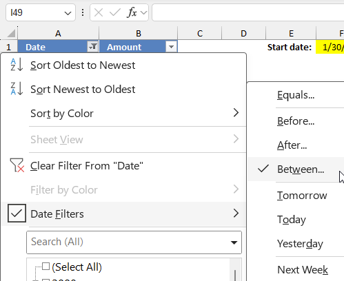
- Press with left mouse button on the arrow next to column header "Date". A popup menu appears.

- Press with left mouse button on "Date Filters", and another menu appears.

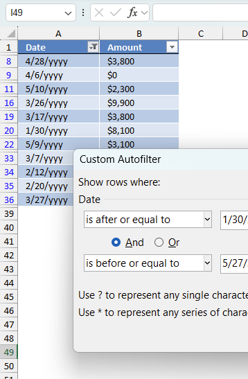
- Press with left mouse button on "Between...".
- A dialog box appears, enter the start and end date.

- Press with left mouse button on the "OK" button to apply changes.
6. Filter rows based on a date range - Advanced filter

This example demonstrates how to filter a data set based on a start and end date using "Advanced Filter". The Advanced Filter in Excel is a powerful tool that allows you to filter data using complex criteria beyond the basic AutoFilter capabilities. Here’s what it does:
- Custom Criteria:
You can set up a criteria range on your worksheet with multiple conditions, including the use of logical operators (AND, OR) and even formulas. - Filter In-Place or to Another Location:
Advanced Filter lets you either filter your data directly within the existing range or copy the filtered results to a different location in your worksheet. - Unique Records:
It provides an option to extract unique records from your data, which is especially useful when dealing with duplicates.
This feature is ideal when you need to perform more refined searches and analyses on your data. Here is what we will do:
- Specify the date range using comparison operators.
- How to start the "Advanced Filter" feature.
- Configure conditions using the dialog box.
- Clear the "Advanced Filter".
6.1 Enter date range
- Enter the column header name containing the dates in cells B2 and C2, they must match. My column header name is "Date" as shown in the image below.

- Type =">=1/30/2025" in cell B3.
- Press Enter.
- Type ="<=5/27/2025" in cell C3.
- Press Enter.
6.2 Start the "Advanced Filter"
- Go to tab "Data" on the ribbon.
- Press with mouse on the button named "Advanced".

- A dialog box appears.

- Select the radio button named "Filter the list, in-place".
- Press with left mouse button on the arrow in "List range:".
- Select cell range B5:C42.
- Press with left mouse button on the arrow in "Criteria range:".
- Select cell range B2:C3.

- Press with left mouse button on the "OK" button.

The blue row numbers show that some sort of filter is applied, in this case, the "Advanced Filter".
6.3 How to clear the "Advanced Filter"
- Go to tab "Data" on the ribbon.
- Press with left mouse button on the button named "Clear".

- The data set goes back to its unfiltered original state.

Filter records category
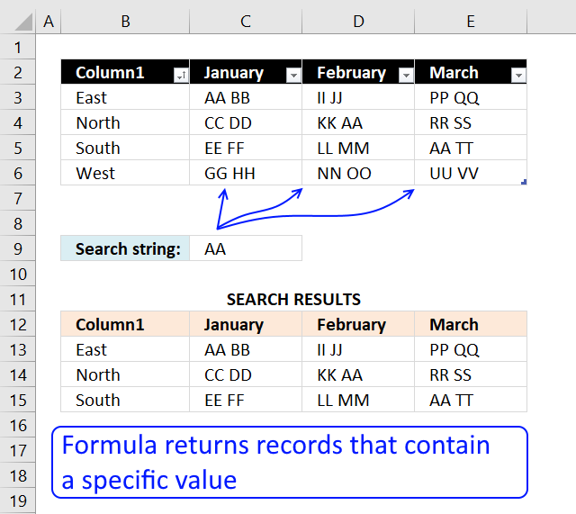
This article explains different techniques that filter rows/records that contain a given text string in any of the cell values […]
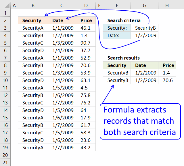
This article demonstrates how to extract records/rows based on two conditions applied to two different columns, you can easily extend […]
Lookup with criteria and return records.
Excel categories
9 Responses to “Extract records between two dates”
Leave a Reply
How to comment
How to add a formula to your comment
<code>Insert your formula here.</code>
Convert less than and larger than signs
Use html character entities instead of less than and larger than signs.
< becomes < and > becomes >
How to add VBA code to your comment
[vb 1="vbnet" language=","]
Put your VBA code here.
[/vb]
How to add a picture to your comment:
Upload picture to postimage.org or imgur
Paste image link to your comment.
This is a great piece of programming, but I cannot for the life of me get it to work in my spread sheet. I have tried naming the ranges, adding dollar signs to keep the references constant, etc., but no matter what I do, it will not filter the date range correctly.
This is the perfect solution to my need, so if there is anything you can do to help me, I would appreciate it. I could send you the spreadsheet if that would help.
Thanks
Tom
Tom,
I have updated the article. Let me know if you got it to work?
Sir
What is table 13 here?
AVIUSHEK,
Table 13 is the table name.
How to find the table name
1.Select your table
2.Press with left mouse button on the "Design" tab on the ribbon
3.Read table name in properties window on the ribbon
I am trying to use your filter-records-between-two-dates.xls Excel 97-2003 Workbook *.xls and use the #num errors removal but the returned value is #NAME? instead, can you tell me what I am doing wrong?
how to add data for Table13
Thanks for tutorial.
I developed a template to filter products between two selected dates using the userform. The filtered products are listed in the listbox. The selected products from the listbox are copied to the other worksheet.
It's image: https://imgur.com/DpkkYDq
To make the date selection easier, I added a date userform (second userform) instead of a calendar control. When press with left mouse button on the textboxes on the main userform, the date userform is opened and the user can easily select the date.
Also, I applied the elongation effect to the userform at the time of filtering.
Source codes and sample file at:https://eksi30.com/filter-products-between-two-dates-with-vba-userform/
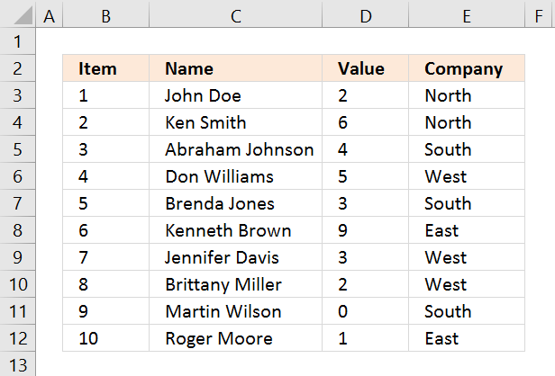
Thank you for the tutorial! I've got this working, but would like to add in another criteria, i.e., return row with date between start date and end date and name = cell value. I added it in the 'if' criteria and get the correct number or rows returned, but not the correct rows. How do I specify this?
Brittany,
Add another logical expression to this formula:
=INDEX($A$2:$B$38, SMALL(IF(($A$2:$A$38<=$H$2)*($A$2:$A$38>=$H$1), MATCH(ROW($A$2:$A$38), ROW($A$2:$A$38)), ""), ROW(A1)), COLUMN(A1))
I have bolded the original logical expressions in the formula above.
If you have a name in cell H3 and names in cells $C$2:$C$38 the formula becomes:
=INDEX($A$2:$C$38, SMALL(IF(($A$2:$A$38<=$H$2)*($A$2:$A$38>=$H$1)*($C$2:$C$38=$H$3), MATCH(ROW($A$2:$A$38), ROW($A$2:$A$38)), ""), ROW(A1)), COLUMN(A1))
Excel 365 users using the example values in section 2 use this formula:
=FILTER(A2:C38,(A2:A38<=H2)*(A2:A38>=H1)*(C2:C38<=H3))