Filter duplicate values based on criteria

This article demonstrates formulas and Excel tools that extract duplicates based on three conditions. The first and second condition is a date range, a start date, and an end date. The third condition is value.
Section 3 below demonstrates how to extract duplicates using the AutoFilter feature, this makes it even easier to apply whatever criteria you want.
Table of Contents
1. Filter duplicate values using criteria

This example demonstrates a formula that works in older Excel versions, I recommend using the Excel 365 formula in section 2 if you have the option. IT is much smaller and easier to understand.
The worksheet, displayed in the image above, allows you to search for duplicate names using a date range (cell C2 and C3) and a condition (cell C4). The result is displayed in cell B7 and cells below.
- The source data range is in E3:G22. It has three columns and their names are:
- Date, City, and Name
- The criteria is in cells C2, C3, and C4:
- Start date, End date, and City
- The retrieved values are in cell B7 and cells below as far as needed. These values are names from G3:G22 and they are duplicates and only duplicate values.
Array formula in cell B7:
The array formula in cell B7 returns two names in this example displayed in cells B7 and B8. The first name is in cells G3, G13, and G17, remember that the date range is 1/1 to 31/1 and the city must be "London". Now only G3 and G17 match. Both values are exactly the same which means that the name is retrieved and displayed in cell B7.
1.1 How to enter an array formula
- Copy (Ctrl + c) the above formula.
- Double press with the left mouse button on cell B7.
- Paste (Ctrl + v) the formula to cell B7.
- Press and hold CTRL + SHIFT simultaneously.
- Press Enter once.
- Release all keys.
Your formula now looks like this: {=array_formula}. Don't enter the curly brackets, they appear automatically. Now copy cell B7 and paste to cells below. Each cell contains a duplicate value.
1.2 Explaining formula in cell A6
Step 1 - Compare end date to dates
The less than sign and the equal sign are logical operators, they let you check if the end date is larger than or equal to dates in cell range $D$2:$D$21.
The output is an array with the same size as the cell range, it contains boolean values TRUE or FALSE.
$E$2:$E$21<=$C$3
becomes
{41275; 41307; 41277; 41337; 41278; 41339; 41311; 41281; 0; 41374; 41307; 41306; 41276; 41337; 41278; 41339; 41311; 41281; 41282; 41374}<=41305
and returns
{TRUE; FALSE; TRUE; FALSE; TRUE; FALSE; FALSE; TRUE; TRUE; FALSE; FALSE; FALSE; TRUE; FALSE; TRUE; FALSE; FALSE; TRUE; TRUE; FALSE}.
Step 2 - Compare start date to dates
$E$2:$E$21>=$C$2
becomes
{41275; 41307; 41277; 41337; 41278; 41339; 41311; 41281; 0; 41374; 41307; 41306; 41276; 41337; 41278; 41339; 41311; 41281; 41282; 41374}<=41275
and returns
{TRUE; TRUE; TRUE; TRUE; TRUE; TRUE; TRUE; TRUE; FALSE; TRUE; TRUE; TRUE; TRUE; TRUE; TRUE; TRUE; TRUE; TRUE; TRUE; TRUE}
Step 3 - Check condition (city)
$F$3:$F$22=$C$4
becomes
{"London";"Paris";"London";"Paris";"London";"Paris";"London";"Paris";0;"London";"London";"Paris";"Paris";"London";"London";"London";"London";"London";"London";"London"}="London"
and returns
{TRUE; FALSE; TRUE; FALSE; TRUE; FALSE; TRUE; FALSE; FALSE; TRUE; TRUE; FALSE; FALSE; TRUE; TRUE; TRUE; TRUE; TRUE; TRUE; TRUE}.
Step 4 - Multiply arrays (AND Logic)
This step applies AND logic to the arrays. This means that both boolean values must be TRUE to return TRUE.
TRUE * TRUE = TRUE, FALSE* TRUE = FALSE, TRUE * FALSE= FALSE, FALSE* FALSE= FALSE.
($D$2:$D$21<=$B$2)*($D$2:$D$21>=$B$1)*($E$2:$E$21=$B$3)
becomes
{TRUE; FALSE; TRUE; FALSE; TRUE; FALSE; FALSE; TRUE; TRUE; FALSE; FALSE; FALSE; TRUE; FALSE; TRUE; FALSE; FALSE; TRUE; TRUE; FALSE} * {TRUE; TRUE; TRUE; TRUE; TRUE; TRUE; TRUE; TRUE; FALSE; TRUE; TRUE; TRUE; TRUE; TRUE; TRUE; TRUE; TRUE; TRUE; TRUE; TRUE} * {TRUE; FALSE; TRUE; FALSE; TRUE; FALSE; TRUE; FALSE; FALSE; TRUE; TRUE; FALSE; FALSE; TRUE; TRUE; TRUE; TRUE; TRUE; TRUE; TRUE}
and returns
{1; 0; 1; 0; 1; 0; 0; 0; 0; 0; 0; 0; 0; 0; 1; 0; 0; 1; 1; 0}.
Note, boolean values are converted into their numerical equivalents when a calculation is made. TRUE = 1 and FALSE = 0 (zero).
Step 5 - Filter values in column F based on criteria
The IF function returns one value if the logical test is TRUE and another value if the logical test is FALSE.
Function syntax: IF(logical_test, [value_if_true], [value_if_false])
IF(($E$3:$E$22<=$C$3)*($E$3:$E$22>=$C$2)*($F$3:$F$22=$C$4), $G$3:$G$22, "")
becomes
IF({1; 0; 1; 0; 1; 0; 0; 0; 0; 0; 0; 0; 0; 0; 1; 0; 0; 1; 1; 0}, {"Latika Turk"; "Aubree Mcintosh"; "Ryann Bartels"; "Jonas Chavis"; "Cliff Oconnor"; "Darla Winters"; "Aubrey Dillard"; "Carina Swafford"; 0; "Jaqueline Shorter"; "Latika Turk"; "Ryann Bartels"; "Jonas Chavis"; "Darla Winters"; "Latika Turk"; "Cliff Oconnor"; "Darla Winters"; "Ryann Bartels"; "Darla Winters"; "Cliff Oconnor"}, "")
and returns
{"Latika Turk"; ""; "Ryann Bartels"; ""; "Cliff Oconnor"; ""; ""; ""; ""; ""; ""; ""; ""; ""; "Latika Turk"; ""; ""; "Ryann Bartels"; "Darla Winters"; ""}
Step 6 - Match filtered values
The MATCH function returns the relative position of an item in an array that matches a specified value in a specific order.
Function syntax: MATCH(lookup_value, lookup_array, [match_type])
MATCH(IF(($E$3:$E$22<=$C$3)*($E$3:$E$22>=$C$2)*($F$3:$F$22=$C$4), $G$3:$G$22, ""), IF(($E$3:$E$22<=$C$3)*($E$3:$E$22>=$C$2)*($F$3:$F$22=$C$4), $G$3:$G$22, "A"), 0)
becomes
MATCH({"Latika Turk"; ""; "Ryann Bartels"; ""; "Cliff Oconnor"; ""; ""; ""; ""; ""; ""; ""; ""; ""; "Latika Turk"; ""; ""; "Ryann Bartels"; "Darla Winters"; ""}, {"Latika Turk"; "A"; "Ryann Bartels"; "A"; "Cliff Oconnor"; "A"; "A"; "A"; "A"; "A"; "A"; "A"; "A"; "A"; "Latika Turk"; "A"; "A"; "Ryann Bartels"; "Darla Winters"; "A"}, 0)
and returns
{1; #N/A; 3; #N/A; 5; #N/A; #N/A; #N/A; #N/A; #N/A; #N/A; #N/A; #N/A; #N/A; 1; #N/A; #N/A; 3; 19; #N/A}.
Step 7 - Filter values based on being a duplicate
The ROW function calculates the row number of a cell reference.
Function syntax: ROW(reference)
IF(MATCH(IF(($D$2:$D$21<=$B$2)*($D$2:$D$21>=$B$1)*($E$2:$E$21=$B$3),$F$2:$F$21,""), IF(($D$2:$D$21<=$B$2)*($D$2:$D$21>=$B$1)*($E$2:$E$21=$B$3), $F$2:$F$21,"A"), 0)<>MATCH(ROW($F$2:$F$21), ROW($F$2:$F$21)), MATCH(ROW($F$2:$F$21), ROW($F$2:$F$21)))
becomes
IF(MATCH({1; #N/A; 3; #N/A; 5; #N/A; #N/A; #N/A; #N/A; #N/A; #N/A; #N/A; #N/A; #N/A; 1; #N/A; #N/A; 3; 19; #N/A}<>{1; 2; 3; 4; 5; 6; 7; 8; 9; 10; 11; 12; 13; 14; 15; 16; 17; 18; 19; 20}, {1; 2; 3; 4; 5; 6; 7; 8; 9; 10; 11; 12; 13; 14; 15; 16; 17; 18; 19; 20})
and returns
{FALSE; #N/A; FALSE; #N/A; FALSE; #N/A; #N/A; #N/A; #N/A; #N/A; #N/A; #N/A; #N/A; #N/A; 15; #N/A; #N/A; 18; FALSE; #N/A}.
Step 8 - Remove error values
The MATCH function returns the relative position of an item in an array that matches a specified value in a specific order.
Function syntax: MATCH(lookup_value, lookup_array, [match_type])
IFERROR({FALSE; #N/A; FALSE; #N/A; FALSE; #N/A; #N/A; #N/A; #N/A; #N/A; #N/A; #N/A; #N/A; #N/A; 15; #N/A; #N/A; 18; FALSE; #N/A}, "")
and returns
{FALSE; ""; FALSE; ""; FALSE; ""; ""; ""; ""; ""; ""; ""; ""; ""; 15; ""; ""; 18; FALSE; ""}.
Step 9 - Extract k-th smallest row number
The SMALL function returns the k-th smallest value from a group of numbers.
Function syntax: SMALL(array, k)
SMALL(IFERROR(IF(MATCH(IF(($D$2:$D$21<=$B$2)*($D$2:$D$21>=$B$1)*($E$2:$E$21=$B$3),$F$2:$F$21,""), IF(($D$2:$D$21<=$B$2)*($D$2:$D$21>=$B$1)*($E$2:$E$21=$B$3), $F$2:$F$21,"A"), 0)<>MATCH(ROW($F$2:$F$21), ROW($F$2:$F$21)), MATCH(ROW($F$2:$F$21), ROW($F$2:$F$21))), ""), ROW(A1))
becomes
SMALL({FALSE; ""; FALSE; ""; FALSE; ""; ""; ""; ""; ""; ""; ""; ""; ""; 15; ""; ""; 18; FALSE; ""}, ROW(A1))
becomes
SMALL({FALSE; ""; FALSE; ""; FALSE; ""; ""; ""; ""; ""; ""; ""; ""; ""; 15; ""; ""; 18; FALSE; ""}, 1)
and returns 15.
Step 10 - Get value based on a row number
The INDEX function returns a value or reference from a cell range or array, you specify which value based on a row and column number.
Function syntax: INDEX(array, [row_num], [column_num])
INDEX($F$2:$F$21, SMALL(IFERROR(IF(MATCH(IF(($D$2:$D$21<=$B$2)*($D$2:$D$21>=$B$1)*($E$2:$E$21=$B$3),$F$2:$F$21,""), IF(($D$2:$D$21<=$B$2)*($D$2:$D$21>=$B$1)*($E$2:$E$21=$B$3), $F$2:$F$21,"A"), 0)<>MATCH(ROW($F$2:$F$21), ROW($F$2:$F$21)), MATCH(ROW($F$2:$F$21), ROW($F$2:$F$21))), ""), ROW(A1)))
becomes
INDEX($F$2:$F$21, 15)
and returns
"Latika Turk".
2. Filter duplicate values using criteria - Excel 365

This example contains an Excel 365 dynamic array formula that automatically spills values to the destination cell and adjacent cells. The source data is in cells E3:G22 just like the example in section 1 above. The criteria is in cells C2:C4 and they are start date, end date, and city.
Excel 365 dynamic array formula in cell B7:
The formula returns two names that have duplicate instances in cells G3:G22 based on the criteria in cells C2:C4. Note that this formula is considerably smaller than the one in section 1. A #SPILL! error occurs if the destination cells are not empty, delete or move the values that hinder the formula and you are good to go.
2.1 Explaining formula
Step 1 - Compare dates to the start date
The less than character and the equal sign combined check if the dates are earlier or equal to the start date.
C2<=E3:E22
becomes
41275<={41275; 41307; 41277; 41337; 41278; 41339; 41311; 41281; 0; 41374; 41307; 41306; 41276; 41337; 41278; 41339; 41311; 41281; 41282; 41374}
and returns
{TRUE; TRUE; TRUE; TRUE; TRUE; TRUE; TRUE; TRUE; FALSE; TRUE; TRUE; TRUE; TRUE; TRUE; TRUE; TRUE; TRUE; TRUE; TRUE; TRUE}.
Step 2 - Compare dates to end date
The greater than character and the equal sign combined check if the dates are later or equal to the start date.
C3>=E3:E22
becomes
41305>={41275; 41307; 41277; 41337; 41278; 41339; 41311; 41281; 0; 41374; 41307; 41306; 41276; 41337; 41278; 41339; 41311; 41281; 41282; 41374}
and returns
{TRUE; FALSE; TRUE; FALSE; TRUE; FALSE; FALSE; TRUE; TRUE; FALSE; FALSE; FALSE; TRUE; FALSE; TRUE; FALSE; FALSE; TRUE; TRUE; FALSE}.
Step 3 - Check the condition
The equal sign checks if the condition is equal to values in cell range F3:F22.
C4=F3:F22
becomes
"London"={"London";"Paris";"London";"Paris";"London";"Paris";"London";"Paris";0;"London";"London";"Paris";"Paris";"London";"London";"London";"London";"London";"London";"London"}
and returns
{TRUE; FALSE; TRUE; FALSE; TRUE; FALSE; TRUE; FALSE; FALSE; TRUE; TRUE; FALSE; FALSE; TRUE; TRUE; TRUE; TRUE; TRUE; TRUE; TRUE}.
Step 4 - Multiply arrays (AND logic)
The asterisk allows you to multiply arrays. The arrays contain either TRUE or FALSE. Multiplying boolean values TRUE or FALSE creates AND - logic meaning both values must be TRUE to return TRUE.
In other words, all three conditions must be met in order to return TRUE.
(C2<=E3:E22)*(C3>=E3:E22)*(C4=F3:F22)
becomes
{TRUE; TRUE; TRUE; TRUE; TRUE; TRUE; TRUE; TRUE; FALSE; TRUE; TRUE; TRUE; TRUE; TRUE; TRUE; TRUE; TRUE; TRUE; TRUE; TRUE} * {TRUE; FALSE; TRUE; FALSE; TRUE; FALSE; FALSE; TRUE; TRUE; FALSE; FALSE; FALSE; TRUE; FALSE; TRUE; FALSE; FALSE; TRUE; TRUE; FALSE} * {TRUE; FALSE; TRUE; FALSE; TRUE; FALSE; TRUE; FALSE; FALSE; TRUE; TRUE; FALSE; FALSE; TRUE; TRUE; TRUE; TRUE; TRUE; TRUE; TRUE}
and returns
{1; 0; 1; 0; 1; 0; 0; 0; 0; 0; 0; 0; 0; 0; 1; 0; 0; 1; 1; 0}.
Step 5 - Filter values based on criteria
The FILTER function filters values in a given cell range based on a condition or criteria.
FILTER(G3:G22, (C2<=E3:E22)*(C3>=E3:E22)*(C4=F3:F22))
becomes
FILTER(G3:G22, {1; 0; 1; 0; 1; 0; 0; 0; 0; 0; 0; 0; 0; 0; 1; 0; 0; 1; 1; 0})
and returns
{"Latika Turk"; "Ryann Bartels"; "Cliff Oconnor"; "Latika Turk"; "Ryann Bartels"; "Darla Winters"}.
The LET function lets you name intermediate calculation results which can shorten formulas considerably and improve performance.
Function syntax: LET(name1, name_value1, calculation_or_name2, [name_value2, calculation_or_name3...])
z - FILTER(G3:G22, (C2<=E3:E22)*(C3>=E3:E22)*(C4=F3:F22))
Step 6 - Match filtered values
The MATCH function returns a number representing the relative position of an item in an array or cell range.
MATCH(z, z, 0)
becomes
MATCH({"Latika Turk"; "Ryann Bartels"; "Cliff Oconnor"; "Latika Turk"; "Ryann Bartels"; "Darla Winters"}, {"Latika Turk"; "Ryann Bartels"; "Cliff Oconnor"; "Latika Turk"; "Ryann Bartels"; "Darla Winters"}, 0)
and returns
{1; 2; 3; 1; 2; 6}.
Step 7 - Create a sequence based on the number of filtered values
The ROWS function calculate the number of rows in a cell range.
Function syntax: ROWS(array)
ROWS(z)
becomes
ROWS({"Latika Turk"; "Ryann Bartels"; "Cliff Oconnor"; "Latika Turk"; "Ryann Bartels"; "Darla Winters"})
and returns
6.
The SEQUENCE function returns a sequence of numbers.
SEQUENCE(rows, [columns], [start], [step])
SEQUENCE(ROWS(z))
becomes
SEQUENCE(6)
and returns
{1; 2; 3; 4; 5; 6}.
Step 8 - Check for duplicates
The less than and greater than characters return TRUE if the numbers don't match indicating that the value is a duplicate.
MATCH(z, z, 0)<>SEQUENCE(ROWS(z))
becomes
{1; 2; 3; 1; 2; 6}<>{1; 2; 3; 4; 5; 6}
and returns
{FALSE; FALSE; FALSE; TRUE; TRUE; FALSE}.
Step 9 - Filter duplicate values
The FILTER function extracts values/rows based on a condition or criteria.
Function syntax: FILTER(array, include, [if_empty])
FILTER(z, MATCH(z, z, 0)<>SEQUENCE(ROWS(z)))
becomes
FILTER({"Latika Turk"; "Ryann Bartels"; "Cliff Oconnor"; "Latika Turk"; "Ryann Bartels"; "Darla Winters"}, {FALSE; FALSE; FALSE; TRUE; TRUE; FALSE})
and returns
{"Latika Turk"; "Ryann Bartels"}.
3. Filter duplicate values using criteria - Autofilter

This example shows how to filter duplicate values using the Autofilter and three conditions. Two conditions are needed to create a date range, start and end date. The third condition is the city.
I need two simple formulas to tell me if a name is visible (not filtered out) and a duplicate. The AutoFilter takes care of the conditions. Here is how:
3.1 Check if the value is hidden/filtered out

This formula shows the value in the adjacent cell to the left if the value is not hidden or not empty.
Formula in cell E3:
Copy cell E3 and paste to cells below as far as needed.
Explaining formula
Step 1 - Check if value is not empty and not hidden
The SUBTOTAL function returns a subtotal from a list or database, you can choose from a variety of arguments that determine what you want the function to do.
Function syntax: SUBTOTAL(function_num, ref1, ...)
SUBTOTAL(3,D3)
Argument 3 represents COUNTA meaning it counts not empty cells. Only cell reference D3 is used, COUNTA will return 1 or 0 (zero) which are the numerical equivalents to TRUE and FALSE respectively.
Step 2 - Show value if not empty and not hidden
The IF function returns one value if the logical test is TRUE and another value if the logical test is FALSE.
Function syntax: IF(logical_test, [value_if_true], [value_if_false])
IF(SUBTOTAL(3,D3),D3,"")
becomes
IF(1,"Latika Turk","")
and returns
"Latika Turk".
3.2 Check if the value is a duplicate

Formula in cell F3:
Copy cell F3 and paste it to the cells below as far as needed.
Explaining formula
Step 1 - Count values in cell range E3:E22 based on condition in cell E3
The COUNTIF function calculates the number of cells that is equal to a condition.
Function syntax: COUNTIF(range, criteria)
COUNTIF($E$3:$E$22,E3)
becomes
=COUNTIF({"Latika Turk";"Aubree Mcintosh";"Ryann Bartels";"Jonas Chavis";"Cliff Oconnor";"Darla Winters";"Aubrey Dillard";"Carina Swafford";"";"Jaqueline Shorter";"Latika Turk";"Ryann Bartels";"Jonas Chavis";"Darla Winters";"Latika Turk";"Cliff Oconnor";"Darla Winters";"Ryann Bartels";"Darla Winters";"Cliff Oconnor"},"Latika Turk")
and returns
3.
Step 2 - Check if the number is larger than 1
The greater than character checks if the number is larger than 1 meaning there are more than one instance of the value.
COUNTIF($E$3:$E$22,E3)>1
becomes
3>1
and returns TRUE.
3.3 Enable Autofilter

Here is how to create an AutoFilter for the data set in cell range B2:F22.
- Select any cell in cell range B2:F22.
- Go to tab "Data" on the ribbon.
- Press with left mouse button on the "Filter" button.

Arrows in the column header appear, they let you apply filters. The next step shows you how.
3.4 Apply Filter criteria

- Press with left mouse button on the arrow next to the column header "Date".
- A popup menu shows up, deselect all checkboxes except "January".
- Press with left mouse button on "OK" button.

- Press with left mouse button on the arrow next to the column header "City".
- A popup menu shows up, deselect all checkboxes except "London".
- Press with left mouse button on the "OK" button.

- Press with left mouse button on the arrow next to the column header "Duplicate?".
- A popup menu shows up, deselect all checkboxes except "TRUE".
- Press with left mouse button on the "OK" button.

Column E now shows all duplicate values.
4. Filter duplicate values using criteria - Excel Table

This example shows how to filter duplicate values using an Excel Table. It is very similar to section 3, however, Excel fills the remaining cells below automatically after you have entered a formula.
Here is how to convert a cell range to an Excel Table.

- Select any cell in the data set.
- Go to tab "Insert" on the ribbon.
- Press with left mouse button on the "Table" button.
- A dialog box appears.
- Press with left mouse button on the "OK" button.

4.1 Enter formulas
See section 3.1 and 3.2 above on how to enter the formulas.

4.2 Apply criteria to Excel Table
Read section 3.4 above on how to filter the Excel Table. The technique is the same for both AutoFilter and the Excel Table.

Duplicate values category
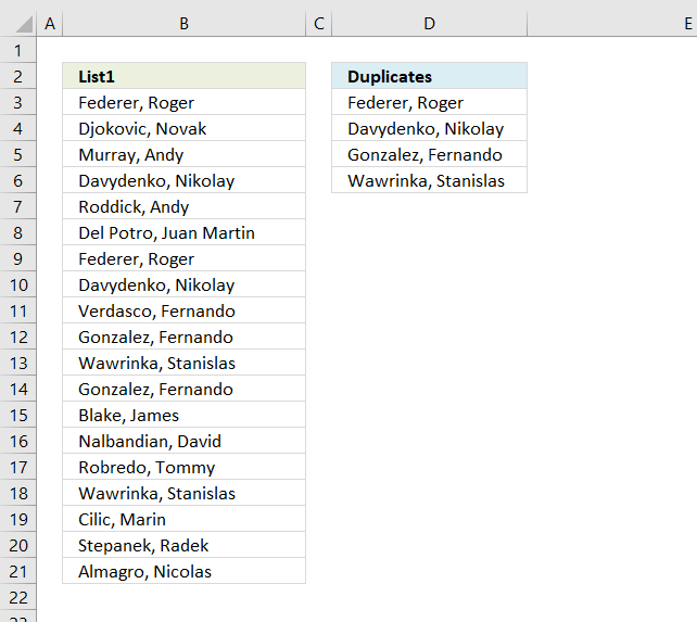
The array formula in cell C2 extracts duplicate values from column A. Only one duplicate of each value is displayed […]
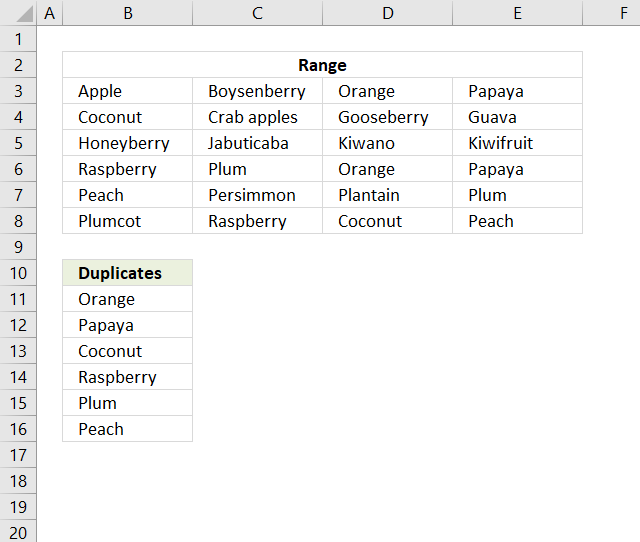
This article describes two formulas that extract duplicates from a multi-column cell range, the first one is built for Excel […]
Excel categories
Leave a Reply
How to comment
How to add a formula to your comment
<code>Insert your formula here.</code>
Convert less than and larger than signs
Use html character entities instead of less than and larger than signs.
< becomes < and > becomes >
How to add VBA code to your comment
[vb 1="vbnet" language=","]
Put your VBA code here.
[/vb]
How to add a picture to your comment:
Upload picture to postimage.org or imgur
Paste image link to your comment.