Dynamic scoreboard

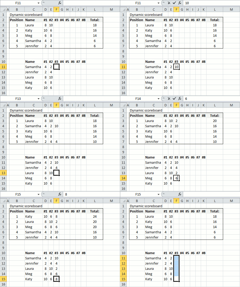
This article demonstrates a scoreboard, displayed to the left, that sorts contestants based on total scores and refreshes instantly each time you enter or edit scores. Section 1 describes a formula for earlier Excel versions than Excel 365, section 2 is
This entire scoreboard is based on formulas only and it is the amazing MMULT function that makes it possible.
The Excel defined Table, shown to the right in the picture above, allows you to enter as many names as you want, no need to update cell references in formulas.
Table of Contents
1. Dynamic scoreboard

Array formula in cell C1:
The formula works even if two or more people share the same total score.
How to enter an array formula
An array formula is a regular formula on steroids, it allows you to perform much more complicated calculations with amazing results.
To enter an array formula you must follow these steps:
- Copy array formula above (CTRL + c).
- Double press with left mouse button on cell C1.
- Paste array formula to the cell.
- Press and hold CTRL + SHIFT simultaneously.
- Press Enter once.
- Release all keys.
If you did it right the formula in the formula bar now begins and ends with curly brackets, like this ={array_formula}. Don't type these characters yourself, they appear if the above steps were correctly done.
Note, if a user edits an array formula and then press Enter key on the keyboard the array formula becomes a regular formula, however, if a user press Esc key on the keyboard the formula returns to an array formula.
This is the single most annoying thing with array formulas, users can easily break them.
How to create an Excel Table
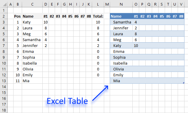
The Excel Table has many useful features, in this case, one specific feature is really great. It allows you to add or delete names to the scoreboard without adjusting cell references, you can have as many names as you like in the Excel Table.
- Select any cell in your data set.
- Press shortcut keys CTRL + T to display the Excel Table dialog box.

- Press with left mouse button on OK button to apply settings and create the table.
Hiding zeros
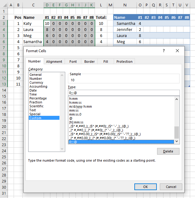
I have applied custom cell formatting to cell range D3:K7 in order to hide 0's (zeros), you can skip these steps if you want them in your worksheet.
- Select cell range D3:K7
- Press short cut keys CTRL + 1 to open the "Format Cells" dialog box.
- Go to tab "Number".
- Press with left mouse button on "Custom" category.
- Type: 0;-0;;@
- Press with left mouse button on OK button to apply cell formatting.
Explaining formula in cell C3
Step 1 - Check if scores are empty
This step creates an array based on cell range D3:K7 and replaces blank values with 0's (zeros).
The less than and greater than characters combined means not equal to and in this case we compare nothing "" meaning an empty cell.
Table2[['#1]:['#8]] is a structured reference pointing to columns #1 to #8 in Table2, Table2 is the name of the Excel Table.
Table2[['#1]:['#8]]<>""
returns
{4, 0, ... , 0}
Step 2 - Create column numbers based on Excel Table headers
The COLUMN function returns a column number based on a cell reference.
COLUMN(Table2[[#Headers], ['#1]:['#8]])
becomes
COLUMN(O2:V2)
and returns {15, 16, 17, 18, 19, 20, 21, 22} which means that the headers are located in column number 15 to 22.
Step 3 - Transpose numbers
The array size is correct, however, all numbers must be 1 to be able to use them in the MMULT function in order to return the desired result. To achieve that we can calculate powers of numbers, in this case power of 0 (zero) which will return 1.
TRANSPOSE(COLUMN(Table2[[#Headers], ['#1]:['#8]])^0)
becomes
TRANSPOSE({15, 16, 17, 18, 19, 20, 21, 22}^0)
becomes
TRANSPOSE({1, 1, 1, 1, 1, 1, 1, 1})
To be able to use the numbers with the MMULT function they need to be separated by semicolons which is easy to accomplish, the TRANSPOSE function changes the array from being arranged horizontally to vertically.
TRANSPOSE({1, 1, 1, 1, 1, 1, 1, 1})
returns {1; 1; 1; 1; 1; 1; 1; 1}
Step 4 - Add numbers column-wise
The MMULT function allows us to sum the numbers horizontally using two arrays.
MMULT(IF(Table2[['#1]:['#8]]<>"", Table2[['#1]:['#8]], 0), TRANSPOSE(COLUMN(Table2[[#Headers], ['#1]:['#8]])^0))
returns {4; 2; 8; 6; 10; 0; 0; 0; 0; 0; 0}. The numbers in the array are in the same order as the names in the Excel Table which is neccessary to be able to sort the names based on scores.
Step 5 - Extract the k-th largest score
The LARGE function calculates the k-th largest number in the array. LARGE(array, k)
LARGE(MMULT(IF(Table2[['#1]:['#8]]<>"", Table2[['#1]:['#8]], 0), TRANSPOSE(COLUMN(Table2[[#Headers], ['#1]:['#8]])^0)), ROWS($A$1:A1))
becomes
LARGE({4; 2; 8; 6; 10; 0; 0; 0; 0; 0; 0}, ROWS($A$1:A1)) returns 10.
The ROWS function contains a cell reference that is both absolute and relative, this makes the cell reference grow when the formula is copied to cells below. This is needed in order to extract a new value in each cell.
Step 6 - Find relative position in array
We have now calculated the k-th largest number in the array and this step explains how to find the position of that value in the array. The MATCH function allows us to do that.
MATCH(LARGE(MMULT(IF(Table2[['#1]:['#8]]<>"", Table2[['#1]:['#8]], 0), TRANSPOSE(COLUMN(Table2[[#Headers], ['#1]:['#8]])^0)), ROWS($A$1:A1)), IF((COUNTIF($C$2:C2, Table2[Name])=0), MMULT(IF(Table2[['#1]:['#8]]<>"", Table2[['#1]:['#8]], 0), TRANSPOSE(COLUMN(Table2[[#Headers], ['#1]:['#8]])^0)), "A"), 0)
becomes
MATCH(10, IF((COUNTIF($C$2:C2, Table2[Name])=0), MMULT(IF(Table2[['#1]:['#8]]<>"", Table2[['#1]:['#8]], 0), TRANSPOSE(COLUMN(Table2[[#Headers], ['#1]:['#8]])^0)), "A"), 0)
becomes
MATCH(10, {4; 2; 8; 6; 10; 0; 0; 0; 0; 0; 0}, 0)
and returns 5. Number 10 is found in position 5 in the array.
Step 7 - Extract the corresponding record to the calculated position
The INDEX function lets you fetch a value based on row and column number.
INDEX(Table2, MATCH(LARGE(MMULT(IF(Table2[['#1]:['#8]]<>"", Table2[['#1]:['#8]], 0), TRANSPOSE(COLUMN(Table2[[#Headers], ['#1]:['#8]])^0)), ROWS($A$1:A1)), IF((COUNTIF($C$2:C2, Table2[Name])=0), MMULT(IF(Table2[['#1]:['#8]]<>"", Table2[['#1]:['#8]], 0), TRANSPOSE(COLUMN(Table2[[#Headers], ['#1]:['#8]])^0)), "A"), 0), COLUMNS($A$1:A1))
becomes
INDEX(Table2, 10, COLUMNS($A$1:A1))
The COLUMNS function chnages when the formula is copied to cells located to the right, this lets us extract the entire record.
INDEX(Table2, 10, COLUMNS($A$1:A1))
becomes
INDEX(Table2, 10, 1)
and returns "Katy" in cell C3.
Step 8 - Remove errors
The IFERROR function removes errors that will show up when all names have been displayed.
IFERROR(INDEX(Table2, MATCH(LARGE(MMULT(IF(Table2[['#1]:['#8]]<>"", Table2[['#1]:['#8]], 0), TRANSPOSE(COLUMN(Table2[[#Headers], ['#1]:['#8]])^0)), ROWS($A$1:A1)), IF((COUNTIF($C$2:C2, Table2[Name])=0), MMULT(IF(Table2[['#1]:['#8]]<>"", Table2[['#1]:['#8]], 0), TRANSPOSE(COLUMN(Table2[[#Headers], ['#1]:['#8]])^0)), "A"), 0), COLUMNS($A$1:A1)), "")
Interested in learning more about array formulas? Join my Advanced Excel Course.
Animated image
The image above shows the scoreboard while I am updating the scores, it sorts the names based on the total.
2. Dynamic scoreboard - Excel 365
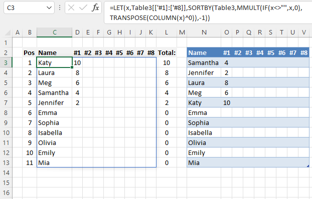
The image above shows
- the Excel 365 formula in cell C3.
- The source data is in cell range N3:V13. In this example, the source range is an Excel defined Table.
The Excel 365 formula aggregates the scores based on each name in cells C3:C13. The score numbers are in cells D3:K13 and each column contains the score of a given round named #1 to #8. The difference with the older formula in section 1 is that this formula spills values to cells below and to the right as far as needed.
Excel 365 lets you use new functions that are better and the formula is a lot shorter. Type the formula in cell C3 and simply press enter. The formula spills to cells below and to the right as far as needed.
Dynamic array formula in cell C3:
Update! Smaller Excel 365 formula
Explaining formula
The following steps shows the larger Excel 365 formula in greater detail.
Step 1 - Check if not empty
Table3[['#1]:['#8]] is a cell reference to data in columns #1 to #8 excluding header names, cell references to Excel Tables are called structured references.
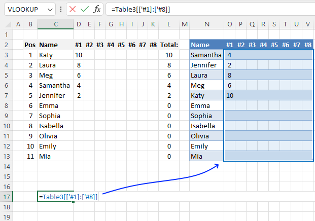
The less than and larger than characters let you perform "not equal to" logic, in this case not equal to nothing. The result is a boolean value, either TRUE or FALSE.
Table3[['#1]:['#8]]<>""
becomes
{4, "", "", ..., ""}<>""
and returns
{TRUE, FALSE, FALSE, ..., FALSE}
Step 2 - Replace empty values with 0 (zero)
The IF function returns one value if the logical test is TRUE and another value if the logical test is FALSE.
Function syntax: IF(logical_test, [value_if_true], [value_if_false])
IF(Table3[['#1]:['#8]]<>"",Table3[['#1]:['#8]],0)
becomes
IF({TRUE, FALSE, FALSE, ..., FALSE},{4, "", "", ..., ""},0)
and returns
{4, 0, 0, ..., 0}.
Step 3 - Create column numbers based on the structured reference
The COLUMN function returns the column number of the top-left cell of a cell reference.
Function syntax: COLUMN(reference)
COLUMN(Table3[['#1]:['#8]])
returns
{15, 16, 17, 18, 19, 20, 21, 22}.
Step 4 - Convert numbers to 1
The caret symbol lets you raise a number to the power of n, in this case, 0 (zero). This results in an array containing 1.
COLUMN(Table3[['#1]:['#8]])^0
and returns {1, 1, 1, 1, 1, 1, 1, 1}
Step 5 - Rearrange horizontal values to vertical
The TRANSPOSE function converts a vertical range to a horizontal range, or vice versa.
Function syntax: TRANSPOSE(array)
TRANSPOSE(COLUMN(Table3[['#1]:['#8]])^0))
and returns {1; 1; 1; 1; 1; 1; 1; 1}
Step 6 - Sum numbers row-wise
The MMULT function calculates the matrix product of two arrays, an array as the same number of rows as array1 and columns as array2.
Function syntax: MMULT(array1, array2)
MMULT(IF(Table3[['#1]:['#8]]<>"",Table3[['#1]:['#8]],0),TRANSPOSE(COLUMN(Table3[['#1]:['#8]])^0))
returns {4; 2; 8; 6; 10; 0; 0; 0; 0; 0; 0}
Step 7 - Sort the table based on the sum
The SORTBY function sorts a cell range or array based on values in a corresponding range or array.
Function syntax: SORTBY(array, by_array1, [sort_order1], [by_array2, sort_order2],…)
SORTBY(Table3,MMULT(IF(Table3[['#1]:['#8]]<>"",Table3[['#1]:['#8]],0),TRANSPOSE(COLUMN(Table3[['#1]:['#8]])^0)),-1)
becomes
SORTBY(Table3,{4; 2; 8; 6; 10; 0; 0; 0; 0; 0; 0},-1)
and returns
{"Katy",10,...,0}
Step 8 - Shorten the formula
The LET function lets you name intermediate calculation results which can shorten formulas considerably and improve performance.
Function syntax: LET(name1, name_value1, calculation_or_name2, [name_value2, calculation_or_name3...])
SORTBY(Table3,MMULT(IF(Table3[['#1]:['#8]]<>"",Table3[['#1]:['#8]],0),TRANSPOSE(COLUMN(Table3[['#1]:['#8]])^0)),-1)
x - Table3[['#1]:['#8]]
LET(x,Table3[['#1]:['#8]],SORTBY(Table3,MMULT(IF(x<>"",x,0),TRANSPOSE(COLUMN(x)^0)),-1))
Get Excel file *.xlsx
Dynamic scoreboard - Excel 365.xlsx
More than 1300 Excel formulasExcel categories
16 Responses to “Dynamic scoreboard”
Leave a Reply
How to comment
How to add a formula to your comment
<code>Insert your formula here.</code>
Convert less than and larger than signs
Use html character entities instead of less than and larger than signs.
< becomes < and > becomes >
How to add VBA code to your comment
[vb 1="vbnet" language=","]
Put your VBA code here.
[/vb]
How to add a picture to your comment:
Upload picture to postimage.org or imgur
Paste image link to your comment.
Oscar -
Great concept - I'll be using this for sure. One question:
You probably had a reason to have the COUNTIF statement and the final COLUMNS. But, by entering the entire non-total row as a single array value you can use the ability of INDEX to return an entire row or column using 0 as the parameter.
=INDEX($C$11:$K$15, MATCH(LARGE(MMULT(IF($D$11:$K$15<>"", $D$11:$K$15,0), ROW(INDIRECT("1:8"))), ROWS($C$11:$C11)), MMULT(IF($D$11:$K$15<>"", $D$11:$K$15, 0), ROW(INDIRECT("1:8"))), 0), 0)
GMF
Thank you, yes the COUNTIF function keeps track of names with the same total score.
Sorry, wordpress eats html characters and I don´t know how to fix it. I edited your formula.
Sorry, the "not equal" values didn't get through the URL encoding. Let's try
=INDEX($C$11:$K$15,MATCH(LARGE(MMULT(IF($D$11:$K$15<>"",$D$11:$K$15,0),ROW(INDIRECT("1:8"))),ROWS($C$11:$C11)),MMULT(IF($D$11:$K$15<>"",$D$11:$K$15,0),ROW(INDIRECT("1:8"))),0),0)OK, I get the COUNTIF saves duplicates! One last time for the INDEX construction i talked about...
=INDEX($C$11:$K$15,MATCH(LARGE(MMULT(IF($D$11:$K$15<>"",$D$11:$K$15,0),ROW(INDIRECT("1:3"))/ROW(INDIRECT("1:3"))),ROWS($C$11:$C11)),(COUNTIF($C$2:C2,$C$11:$C$15)=0)*MMULT(IF($D$11:$K$15<>"",$D$11:$K$15,0),ROW(INDIRECT("1:3"))/ROW(INDIRECT("1:3"))),0),0)I'll bet there's a cleaner way to generate an array of 1's for the MMULT function to cope with flexible numbers of columns for calculating the total, but I couldn't think of it right away!
Here is what I did to create the one's vector
=INDEX($C$11:$K$15,MATCH(LARGE(MMULT(IF($D$11:$K$15"",$D$11:$K$15,0),(1+0*ROW(OFFSET(INDIRECT("A1"),0,0,COUNTA($D$10:$K$10),1)))),ROWS($A$3:B3)),(COUNTIF($C$2:D2,$C$11:$C$15)=0)*MMULT(IF($D$11:$K$15"",$D$11:$K$15,0),(1+0*ROW(OFFSET(INDIRECT("A1"),0,0,COUNTA($D$10:$K$10),1)))),0),COLUMNS($A$3:B3))
Can the above formula be used for 100 tables for 10 rounds? What would the formula to carry this out?
Instead of just 5 how would I do this for 50 people?
I need help developing onto your dynamic scoreboard. I would like it to be 50 down and 50 across. Please help.
Hi Oscar very clever how would I alter it to manage the score of 16 people?
Charles Clarke
Array formula in cell C3:
=INDEX($C$21:$K$36, MATCH(LARGE(MMULT(IF($D$21:$K$36<>"", $D$21:$K$36, 0), {1; 1; 1; 1; 1; 1; 1; 1}), ROWS($A$1:A1)), (COUNTIF($C$2:C2, $C$21:$C$36)=0)*MMULT(IF($D$21:$K$36<>"", $D$21:$K$36, 0), {1; 1; 1; 1; 1; 1; 1; 1}), 0), COLUMNS($A$1:A1))
Dynamic-scoreboard_Charles.xlsx
Charles Clarke,
I have now changed this article so any number of people can be managed.
Hello Oscar, i`d like to start by thanking you for posting this scoreboard - however i found myself in a pickle with altering it for a larger scale, been at it for a few days now - and I`ll really need your help for this:
The required scale will be from #1 - #31 and Position will be for 130 names, will you be able to help with a draft for that ?
Hello Oscar, would you be so kind to help me scale this to this format in a draft?
#1 to #31
and names 130 downwards?
been at this for days now and it`s not working ?
Alexandru
Hard to say. Can you post your formula?
Great Scoreboard. How would I reverse the scoreboard with the lowest score at the top of the table for Golf, which is based on the winner with lowest score?
The third argument in the SORTBY function lets you specify the sort order. 1 - Ascending Large to small. -1 - Descending Small to large