Create a dynamic named range

What is a named range? A named range is a feature in Excel that allows you to assign a specific name to a specific cell or a cell range, or even a formula. If cell A1 contains a specific value that you want to use in multiple formulas you can assign it a descriptive name which allows the formulas to be more intuitive and easier to understand.

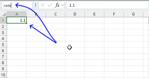
For example, cell A1 contains 1.1 which is a rate. You can assign name "rate" to cell A1 and use "rate" in the formulas. =rate*B2 The easiest way to assign a cell is to select the cell, then press with left mouse button on the "Name box". A prompt appears, type the name and then press Enter.

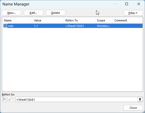
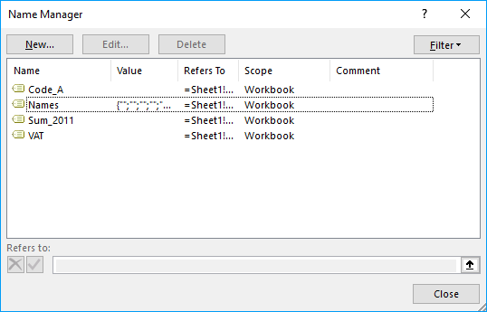
You can find all your named ranges in the "Name Manager". Here is how to access the "Name Manager". Go to tab "Formulas" on the ribbon. Press with mouse on "Name Manager" button, a dialog box appears. See the image above.

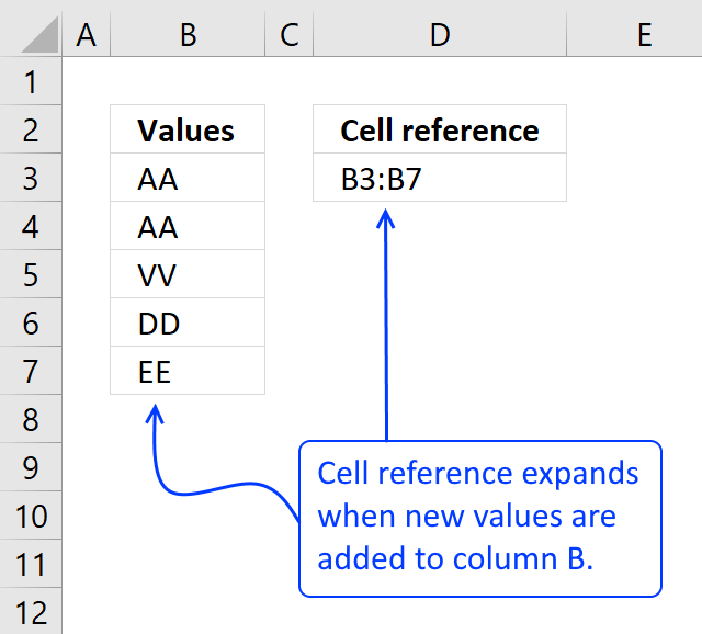
What is a dynamic named range? A dynamic named range grows automatically when new values are added and also shrinks if values are deleted. This saves you time as you no longer need to adjust the cell reference in a formula.

So how does this work? As I told you before, you can also use a formula in a named range. The formula calculates how many cells are populated and returns a cell reference that you can use in another formula.

What is the benefit of using a dynamic named range? This technique makes it easier to use formulas as you don't need to manually adjust their cell references as new values are being entered.

What is an Excel 365 dynamic array? It is a a new feature, for formula, available only to Excel 365 subscribers that automatically spills values to adjacent cells if needed. There is no need anymore for entering array formulas as we used to do in earlier Excel versions. This also makes named ranges redundant in specific cases because referencing dynamic arrays is simply done by adding a hashtag after the cell reference. For example, =A1# references the formula in cell A1 and all spilled values even if the number of values change. I will go in to detail about this in section 1 below.

What other Excel features use dynamic cell references? Excel defined Tables also uses dynamic cell references, however, they are called "structured references". The Excel Table grows or shrinks depending what you do to your data, structured references does not change. They stay the same as long as you don't change their names. The structured reference contains a table name, a column name and sometimes a row specifier. For example Table1[Name][#All].

1. Dynamic arrays - Excel 365

Dynamic arrays are a powerful feature introduced in Excel 365 that automatically spill results into multiple cells when a formula returns more than one value. This is a significant change from how arrays worked in previous Excel versions. Let me explain the key differences:

Dynamic Arrays in Excel 365:

1. Automatic spilling: Formulas that return multiple results automatically expand into neighboring cells.
2. No need for Ctrl+Shift+Enter: You don't need to enter array formulas with a special key combination.
3. Dynamic resizing: The result range automatically adjusts if the source data changes.
4. New functions: Introduced several new functions like SORT, FILTER, UNIQUE, and SEQUENCE.

Easier to use: Simplifies many complex operations that previously required multiple steps.

Working with arrays in previous Excel versions:

1. Manual array entry: Required Ctrl+Shift+Enter to create array formulas.
2. Fixed size: Array formulas had to be entered into a pre-selected range.
3. Less flexible: Changing array size often required manual adjustment.
4. Limited built-in array functions: Fewer functions designed specifically for array operations.
5. More complex: Many array operations required intricate formulas or helper columns.

These changes make working with arrays in Excel 365 much more intuitive and powerful. The image demonstrates a basic use of dynamic arrays in Excel 365. Let me explain the key elements:

1. Dynamic Array formula in cell B5:
   =SEQUENCE(C2)

   SEQUENCE is a new function in Excel 365 that generates a sequence of numbers. It's using the value in C2 (which is 5) to determine how many numbers to generate. The result "spills" automatically down from B5 to B9, creating a dynamic array of numbers from 1 to 5.

2. The area from B5 to B9 is called a spill range. Excel automatically expands the result to fill the necessary cells. This happens without the need to pre-select a range or use special key combinations (like Ctrl+Shift+Enter in older Excel versions).
3. Referencing Dynamic Arrays. In cell C11, the formula
   =COUNT(B5#)

   is used. The # symbol is called the spill range operator. It refers to the entire dynamic array that starts in B5. This allows you to perform operations on the whole array without needing to specify the exact range.

4. Flexibility or what makes the array dynamic: If you change the value in C2, the SEQUENCE function will automatically adjust, and the spill range will expand or contract accordingly. The COUNT function in C11 will also automatically update to reflect the new array size.

This example showcases how dynamic arrays in Excel 365 make it easier to work with ranges that might change size which is often the case in Excel 365. The formulas are simpler, more intuitive, and automatically adjust to data changes, making spreadsheets more dynamic and easier to maintain.

Can you use a cell reference to an Excel 365 dynamic array as a Pivot Table data source? Yes, you can. However, the cell reference, for example =I3# changes to I3:J6 automatically which makes the whole point useless. The reason we want to use an Excel 365 dynamic array reference is to make the Pivot Table also dynamic meaning it includes new values automatically.

I recommend converting the data to an Excel Table and then use a structured reference to the Excel Table as the data source. Note, you still need to "refresh" the Pivot Table to adjust for changes in the source data which is easy to forget.

Here is how to refresh the Pivot Table data source:

1. Press with right mouse button on on any cell in the Pivot Table, a pop up menu appears.
2. Press with mouse on "Refresh".

Here is how to adjust the Pivot Table data source:

1. Select any cell in the Pivot Table.
2. Go to tab "PivotTable Analyze" on the ribbon.
3. Press with left mouse button on "Change Data Source" button.
   
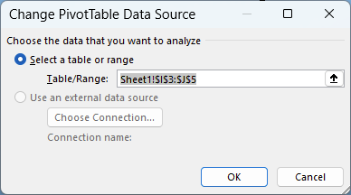
   A dialog box appears.
4. Change the "Table/Range" accordingly.
5. Press with left mouse button on the "OK" button to apply changes.

What about an Excel 365 dynamic array reference in a Drop-down list?

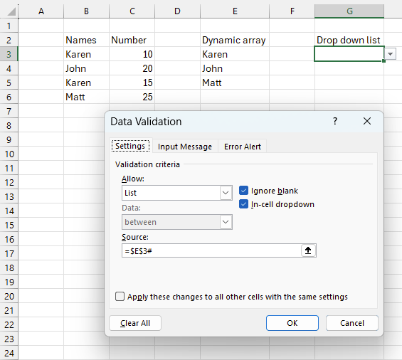
No problem, it works fine. The drop-down list instantly updates if the source data is changed. The image above shows the settings for a drop-down list in cell G3.

Here is how to create a drop-down list with an Excel 365 dynamic array reference:

1. Select the cell that contains the drop-down list.
2. Go to tab "Data" on the ribbon.
3. Press with left mouse button on the "Data Validation" button.
4. Change the drop-down list below "Allow:" to "List".
5. Change the cell reference below "Source:" to an Excel 365 dynamic array reference meaning it ends with a hashtag.
6. Press with left mouse button on "OK" button.

Can I use an Excel 365 dynamic array formula in an Excel Table? Yes and no. Here are two examples:

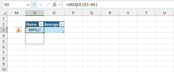
The first example, shown in the image above demonstrates an Excel Table in cells N2:O3. Cell N3 contains an Excel 365 dynamic array that spills values to adjacent cells. The Excel defined Table won't resize based on spilled values, the cell returns "SPILL!" error.

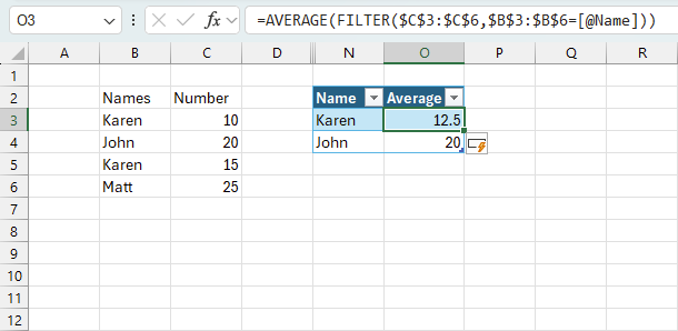
The second example displayed in the image above shows the same Excel defined Table, however, the Excel 365 formula in cell O3 returns a single value which is accepted. The formula calculates the average of the numbers in column C based on the name on the same row.

1.1 Reference dynamic arrays in charts

Excel charts will not allow dynamic arrays unfortunately as shown in the image above, however, there is a workaround. Yes, you guessed it: Named range.

The clip above shows a chart that dynamically resizes when cell F2 changes. Cell F2 determines the number of rows in cell B3 and below and also cell C3 and cells below. Here is how to build it:

1. Go to tab "Formulas".
2. Press with mouse on "Name Manager". A dialog box appears.
3. Press with left mouse button on "New..." button. Another dialog box appears.
4. Specify a name and specify the source cell of the dynamic array using the # hashtag symbol. For example, the demo above uses these names and cell references:
   Name: rand, Refers to: ='Dynamic arrays - chart'!$C$3#
   Name: seq, Refers to: ='Dynamic arrays - chart'!$B$3#
5. Press with left mouse button on the "Close" button to dismiss the "Name Manager" dialog box.

We now need to set up the chart:

1. Create a chart.
2. Press with right mouse button on on the chart, a popup menu appears.
3. Select "Select Data...". A dialog box shows up named "Select Data Source".
   
4. Press with left mouse button on the "Edit" buttons to edit Edit the "Series" and "Axis" values. I am using the following values as source references:
   ='Create a dynamic named range.xlsx'!rand
   ='Create a dynamic named range.xlsx'!seq
   
   
5. Press with left mouse button on the "OK" button to dismiss the dialog box.

Change the value in cell F2 and the chart changes instantly.

2. Create a dynamic named range

In this section, I am going to explain the dynamic named range formula in Sam's comment. The formula adds new rows and columns instantly to the named range. This makes the named range dynamic meaning you don't need to adjust cell references every time you add a new row or column to the list. The formula takes care of only one list per sheet.

How to create a named range

1. Press with left mouse button on the "Formulas" tab on the ribbon.
2. Press with left mouse button on "Name Manager" button, a dialog box "Name Manager" appears.
3. Press with left mouse button on "New..." button to create a new named range and name it.
4. Type the formula below in "Refers to:" window:
   
5. Press with left mouse button on the "Close" button.

Named range formula

Back to top

2.1 Explaining formula

Step 1 - Count non-empty cells in column A

The COUNTA function counts non-empty cells in a given cell range or array.

COUNTA(value1, [value2], ...)

COUNTA($A:$A)

returns 3. There are three values in column A.

Step 2 - Count non-empty cells in row 1

COUNTA($1:$1)

returns 4. There are four values in row 1.

Step 3 - Create cell reference to last non-empty cell

The INDEX function returns a value based on a row and column number, however, it can also be used to create a cell reference.

INDEX(array, [row_num], [column_num], [area_num])

INDEX($1:$1048576, COUNTA($A:$A), COUNT($1:$1))

becomes

INDEX($1:$1048576, 3, 4)

and returns D3.

Step 4 - Create cell reference to the entire cell range

The colon character lets you combine two cell references and create a larger cell ref to a cell range.

$A$1:INDEX($1:$1048576, COUNTA($A:$A), COUNT($1:$1))

and returns $A$1:$D$3.

Back to top

When to use named ranges?

• Formulas, making them dynamic and easier to read and understand.
• Charts (How to create a dynamic chart)
• Pivot tables (Create a dynamic pivot table and refresh automatically in excel)

Back to top

3. List all named ranges and their cell references

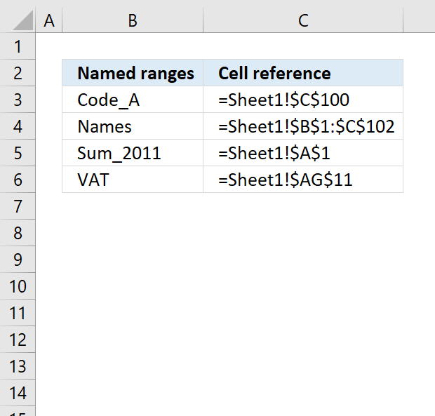
This article shows you a way to display all named ranges you have in a workbook. This is a powerful feature in Excel if you have many named ranges and Excel defined tables and you want a better overview.

Instructions on how to build a list with all your named ranges:

1. Go to "Formula" tab on the ribbon.
2. Press with mouse on "Use in Formula" button on the ribbon.
3. Press with mouse on "Paste Names...", a dialog box appears.
4. Press with left mouse button on "Paste List" button on the dialog box.
5. The list of named ranges is created.

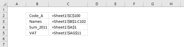
The image below shows the named ranges in the "Name Manager" dialog box, they correspond to the list show in the image above.

Back to top

Named range category

More than 1300 Excel formulas

Excel categories

Comments (11)