How to use the SYD function
What is the SYD function?
The SYD function calculates the yearly asset depreciation of a given year.
Table of Contents
1. Introduction
What is SYD function an abbreviation of?
SYD stands for the "Sum-of-the-Years-Digits" depreciation method, which is a way of calculating depreciation such that the charges decrease each year over an asset's lifespan.
What is the "Sum-of-the-Years-Digits" depreciation method?
The sum-of-the-years-digits (SYD) method is a way to calculate depreciation such that the charges decrease each year over an asset's lifespan.
For example, say an asset has a 5 year life. The SYD fractions for each year would be:
Year 1: 5/15
Year 2: 4/15
Year 3: 3/15
Year 4: 2/15
Year 5: 1/15
(Sum 1+2+3+4+5 = 15)
Depreciation in year 1 is (Cost-salvage) * 5/15, in year 2 it's (Cost-salvage) * 4/15, becoming smaller each year.
What is depreciation of an asset?
Depreciation is an accounting method that allows businesses to allocate the cost of a tangible asset over its useful life. It represents how much of an asset’s value has been used up over time.
Depreciation helps businesses to match their expenses with their revenues, and to reduce their taxable income by deducting the depreciation expense.
What is a depreciable asset?
A depreciable asset is a long-term tangible or physical asset like machinery or equipment that loses value over time due to wear and tear from usage. Depreciation allows a business to recover the cost of the asset as an expense over its useful lifespan.
What is the difference between DB function and the SYD function?
The DB function calculates the fixed-declining balance depreciation each period using a fixed rate, while SYD calculates the sum-of-the-years-digits depreciation based on a declining charge-off fraction each period.
What is the difference between DDB function and the SYD function?
DDB uses fixed declining percentages of the book value to calculate depreciation each period, while SYD calculates the sum-of-the-years-digits depreciation based on a declining charge-off fraction each period.
Depreciation functions in Excel
| Function | Description |
|---|---|
| SYD(cost, salvage, life, period) | Sum-of-the-years digits depreciation |
| DB(cost, salvage, life, period, [month]) | Fixed-declining balance depreciation |
| DDB(cost, salvage, life, period, [factor]) | Double-declining balance depreciation |
| AMORLINC(cost, date_purchased, first_period, salvage, period, rate, [basis]) | Depreciation for period using linear method |
| AMORDEGRC(cost, date_purchased, first_period, salvage, period, rate, [basis]) | Depreciation from date of purchase to end of period |
| VDB(cost, salvage, life, start_period, end_period, [factor], [no_switch]) | Variable declining balance depreciation |
What is the math formula behind this function?
The math formula for the SYD function is:
((cost - salvage) * (life - per + 1) * 2) / (life * (life + 1))
- cost: The initial cost of the asset.
- salvage: The estimated salvage value (value at the end of the asset's useful life) of the asset.
- life: The number of periods over which the asset is being depreciated (useful life).
- per: The period for which you want to calculate the depreciation. Per must use the same units as life.
The formula calculates the depreciation for a given period by first determining the total depreciable cost (cost - salvage). It then applies a fraction based on the remaining useful life of the asset (life - per + 1) and a scaling factor (2 / (life * (life + 1))) to distribute the depreciable cost over the asset's useful life using the Sum-of-Years' Digits method.
2. Syntax
SYD(cost, salvage, life, per)
| cost | Required. The cost of an asset. |
| salvage | Required. The final value after depreciation (salvage value). |
| life | Required. The number of periods the asset is depreciated. |
| per | Required. The period you want to know the depreciation for. |
What is salvage value?
Salvage value is the estimated value of an asset at the end of its useful life. It is also known as scrap value or residual value. It is used to calculate the depreciation expense of an asset over its useful life.
3. Example 1
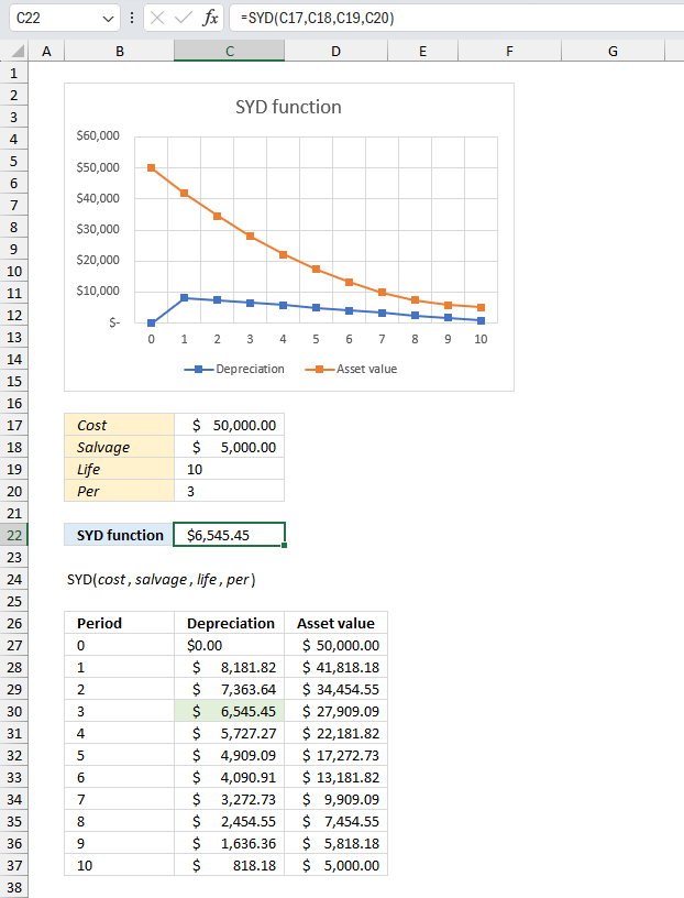
A company purchased a machinery for $50,000 with an estimated salvage value of $5,000 and a useful life of 10 years. Calculate the depreciation for the 3rd year using the Sum-of-Years' Digits method?
This image above shows this example of calculating the depreciation of an asset using the Sum-of-Years' Digits method.
The arguments provided are:
- Cost: $50,000.00
- Salvage: $5,000.00
- Life: 10 years
- Per: 3 (indicating the depreciation calculation for the 3rd year)
Formula in cell C22:
The formula in cell C22 returns $6,545.45 which represents the depreciation value for period 3 (year 3).
The chart displays the depreciation and asset value over the asset's useful life. The blue line represents the depreciation value which starts high and decreases each year. The orange line represents the asset value which starts at the initial cost and decreases as depreciation is applied.
The table below the formula shows the depreciation values and remaining asset values for each period (year) in the asset's useful life.
The math formula for the SYD function is:
((cost - salvage) * (life - per + 1) * 2) / (life * (life + 1))
Lets plug the argument values in this math formula and see what we get.
= ((50,000 - 5,000) * (10 - 3 + 1) * 2) / (10 * (10 + 1))
= (45,000 * 8 * 2) / (10 * 11)
= 720,000 / 110
= 6,545.45
This matches the value displayed in cell C22 and the depreciation value for period 3 (year 3) in the table.
4. Example 2

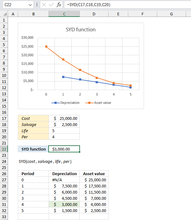
A vehicle costing $25,000 with an estimated salvage value of 10%, is expected to have a useful life of 5 years. Find the depreciation for the 4th year using the Sum-of-Years' Digits method?
This image above shows this example of calculating the depreciation of an asset using the Sum-of-Years' Digits method.
The arguments provided are:
- Cost: $25,000.00
- Salvage: $2,500.00 (10% salvage value)
- Life: 5 years
- Per: 4 (indicating the depreciation calculation for the 4th year)
Formula in cell C22:
The formula in cell C22 returns $3,000.00 which represents the depreciation value for period 4 (year 4).
The chart displays the depreciation and asset value over the asset's useful life. The blue line represents the depreciation value which starts high and decreases each year. The orange line represents the asset value which starts at the initial cost and decreases as depreciation is applied.
The table below the formula shows the depreciation values and remaining asset values for each period (year) in the asset's useful life, from period 0 (zero) to 5.
The math formula for the SYD function is:
((cost - salvage) * (life - per + 1) * 2) / (life * (life + 1))
Lets plug the argument values in this math formula and see what we get.
= ((25,000 - 2,500) * (5 - 4 + 1) * 2) / (5 * (5 + 1))
= (22,500 * 2 * 2) / (5 * 6)
= 3000
5. Function not working
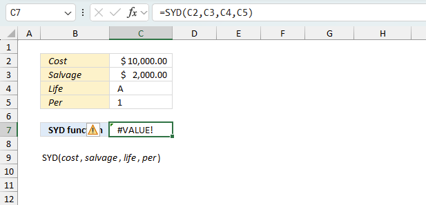
- The SYD function returns a #VALUE! error if a nonnumerical value is used in any of the arguments.
- It propagates error values and returns the same error value.
- A #NAME? error is displayed if you misspell the function name.
5.1 Troubleshooting the error value
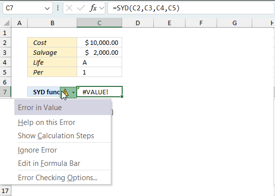
When you encounter an error value in a cell a warning symbol appears, displayed in the image above. Press with mouse on it to see a pop-up menu that lets you get more information about the error.
- The first line describes the error if you press with left mouse button on it.
- The second line opens a pane that explains the error in greater detail.
- The third line takes you to the "Evaluate Formula" tool, a dialog box appears allowing you to examine the formula in greater detail.
- This line lets you ignore the error value meaning the warning icon disappears, however, the error is still in the cell.
- The fifth line lets you edit the formula in the Formula bar.
- The sixth line opens the Excel settings so you can adjust the Error Checking Options.
Here are a few of the most common Excel errors you may encounter.
#NULL error - This error occurs most often if you by mistake use a space character in a formula where it shouldn't be. Excel interprets a space character as an intersection operator. If the ranges don't intersect an #NULL error is returned. The #NULL! error occurs when a formula attempts to calculate the intersection of two ranges that do not actually intersect. This can happen when the wrong range operator is used in the formula, or when the intersection operator (represented by a space character) is used between two ranges that do not overlap. To fix this error double check that the ranges referenced in the formula that use the intersection operator actually have cells in common.
#SPILL error - The #SPILL! error occurs only in version Excel 365 and is caused by a dynamic array being to large, meaning there are cells below and/or to the right that are not empty. This prevents the dynamic array formula expanding into new empty cells.
#DIV/0 error - This error happens if you try to divide a number by 0 (zero) or a value that equates to zero which is not possible mathematically.
#VALUE error - The #VALUE error occurs when a formula has a value that is of the wrong data type. Such as text where a number is expected or when dates are evaluated as text.
#REF error - The #REF error happens when a cell reference is invalid. This can happen if a cell is deleted that is referenced by a formula.
#NAME error - The #NAME error happens if you misspelled a function or a named range.
#NUM error - The #NUM error shows up when you try to use invalid numeric values in formulas, like square root of a negative number.
#N/A error - The #N/A error happens when a value is not available for a formula or found in a given cell range, for example in the VLOOKUP or MATCH functions.
#GETTING_DATA error - The #GETTING_DATA error shows while external sources are loading, this can indicate a delay in fetching the data or that the external source is unavailable right now.
5.2 The formula returns an unexpected value
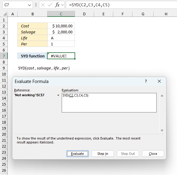
To understand why a formula returns an unexpected value we need to examine the calculations steps in detail. Luckily, Excel has a tool that is really handy in these situations. Here is how to troubleshoot a formula:
- Select the cell containing the formula you want to examine in detail.
- Go to tab “Formulas” on the ribbon.
- Press with left mouse button on "Evaluate Formula" button. A dialog box appears.
The formula appears in a white field inside the dialog box. Underlined expressions are calculations being processed in the next step. The italicized expression is the most recent result. The buttons at the bottom of the dialog box allows you to evaluate the formula in smaller calculations which you control. - Press with left mouse button on the "Evaluate" button located at the bottom of the dialog box to process the underlined expression.
- Repeat pressing the "Evaluate" button until you have seen all calculations step by step. This allows you to examine the formula in greater detail and hopefully find the culprit.
- Press "Close" button to dismiss the dialog box.
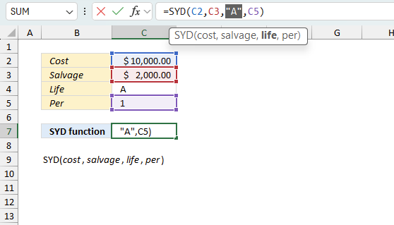
There is also another way to debug formulas using the function key F9. F9 is especially useful if you have a feeling that a specific part of the formula is the issue, this makes it faster than the "Evaluate Formula" tool since you don't need to go through all calculations to find the issue..
- Enter Edit mode: Double-press with left mouse button on the cell or press F2 to enter Edit mode for the formula.
- Select part of the formula: Highlight the specific part of the formula you want to evaluate. You can select and evaluate any part of the formula that could work as a standalone formula.
- Press F9: This will calculate and display the result of just that selected portion.
- Evaluate step-by-step: You can select and evaluate different parts of the formula to see intermediate results.
- Check for errors: This allows you to pinpoint which part of a complex formula may be causing an error.
The image above shows cell reference C4 converted to hard-coded value using the F9 key. The SYD function requires numerical values in any argument which is not the case in this example. We have found what is wrong with the formula.
Tips!
- View actual values: Selecting a cell reference and pressing F9 will show the actual values in those cells.
- Exit safely: Press Esc to exit Edit mode without changing the formula. Don't press Enter, as that would replace the formula part with the calculated value.
- Full recalculation: Pressing F9 outside of Edit mode will recalculate all formulas in the workbook.
Remember to be careful not to accidentally overwrite parts of your formula when using F9. Always exit with Esc rather than Enter to preserve the original formula. However, if you make a mistake overwriting the formula it is not the end of the world. You can “undo” the action by pressing keyboard shortcut keys CTRL + z or pressing the “Undo” button
5.3 Other errors
Floating-point arithmetic may give inaccurate results in Excel - Article
Floating-point errors are usually very small, often beyond the 15th decimal place, and in most cases don't affect calculations significantly.
Functions in 'Financial' category
The SYD function function is one of 27 functions in the 'Financial' category.

How to comment
How to add a formula to your comment
<code>Insert your formula here.</code>
Convert less than and larger than signs
Use html character entities instead of less than and larger than signs.
< becomes < and > becomes >
How to add VBA code to your comment
[vb 1="vbnet" language=","]
Put your VBA code here.
[/vb]
How to add a picture to your comment:
Upload picture to postimage.org or imgur
Paste image link to your comment.
Contact Oscar
You can contact me through this contact form