How to use the MINA function

What is the MINA function?

The MINA function returns the smallest number from an array or cell range. Blank cells are ignored, boolean value TRUE evaluates to 1 and FALSE to 0 (zero). Text values are also evaluated to 0 (zero).

1. Introduction

What is MINA an abbreviation of?

MINA stands for minimum alternative or minimum all meaning it also evaluates logical values and text as numbers. Text and boolean value FALSE is evaluated to 0 (zero), boolean value TRUE is 1.

What is the difference between the MIN function and the MINA function?

The MIN function excludes or ignores blank cells, text and boolean values. The MINA function ignores blank cells, includes text and boolean values. Text values are evaluated as 0 (zero), boolean value TRUE is 1 and boolean value FALSE is 0 (zero).

Related functions

Function	Description
MIN(number1,number2,...)	Returns the smallest numeric value
MINA(value1,value2,...)	Returns the smallest value including text
MINIFS(min_range, criteria_range1, criteria1,...)	Returns min from a range meeting multiple criteria
SMALL(array, k)	Returns the k-th smallest value in array
AGGREGATE(4,options,array,k)	Returns k-th smallest value ignoring hidden rows/columns
DMIN(database, field, criteria)	Returns min value in a database meeting criteria

When is the MIN function useful in statistics?

The MIN function allows you to find the minimum or lowest value in a set of data points. This can be helpful when you want to identify outliers or extreme values in your dataset.

The range of a dataset is the difference between the maximum and minimum values. You can use the MIN function in combination with the MAX function to calculate the range which is a measure of the spread of the data.

2. Syntax

MINA(value1, [value2], ...)

3. Arguments

value1	Required. Value or cell ref for which you want to find the smallest number.
[value2]	Optional. Up to 254 additional arguments.

4. Example 1

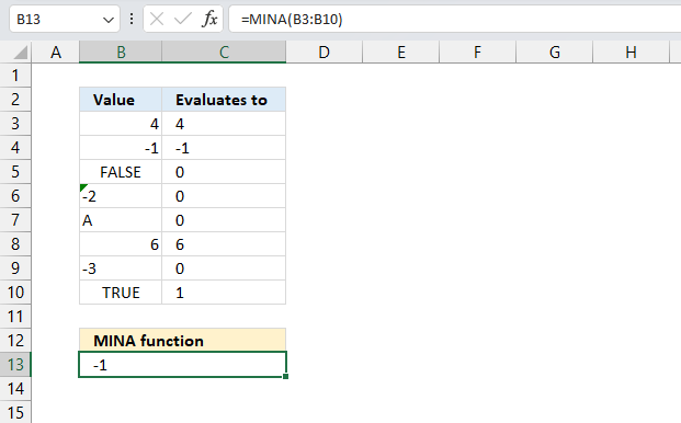
This example demonstrates how the MINA function works. Cell range B3:B10 contains values, the corresponding cells in C3:C10 shows how the MINA function "evaluates" these values.

Excel aligns values to the right if it is recognized as a number or numerical value. Excel aligns values to the left if Excel "evaluates" the value as a text value. The image above shows that Excel thinks that -2 is a text value. This can happen if you work with imported data from other sources like databases, the web etc.

Boolean values and error values are center aligned, FALSE in cell B5 is 0 (zero) and TRUE om cell B10 is 1.

Formula in cell B13:

The formula in cell B13 returns -1 which is the smallest number in cell range B3:B10. How do you convert numerical values stored as text values in Excel? Excel often labels the cell with a green arrow in the top left corner. Select the cell and a box containing an exclamation mark shows up.

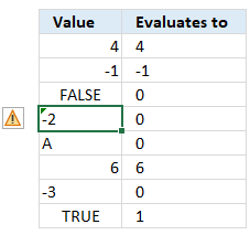
Press with left mouse button on the exclamation mark and popup appears containing available options.

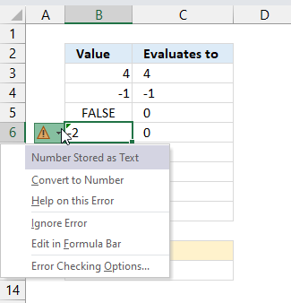
Select the second row "Convert to number" to do the obvious thing convert the value to a number. You also have the option to get more information about this particular error. You can also ignore the error entirely.

5. Example 2

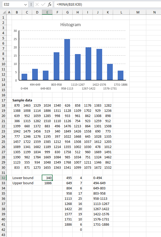
In a manufacturing quality control process, the number of defects found in 130 randomly selected days during a year were:

870	1463	1529	1024	1540	626	858	1176	1383	1282
1388	1008	1114	1886	1311	1128	1109	1702	929	1236
639	952	1059	1285	998	933	961	862	1308	898
386	1315	1282	1510	1110	1126	754	923	1259	912
1399	660	1372	883	496	1476	1213	864	1301	1508
1042	1479	1456	519	340	1849	1426	1558	690	773
777	1246	1276	1195	397	1022	1668	645	1028	1335
1457	1722	1559	1585	1212	934	1508	1037	1612	1205
1089	1341	1682	1189	1214	1355	1002	1030	478	1012
1305	1199	1834	999	830	1758	512	960	1669	1491
1390	982	1784	1669	1084	985	1034	751	1324	1462
1123	555	934	1048	1549	1768	1007	1211	1346	862
833	871	1273	1655	1563	1541	1099	1073	1672	1532

Build a frequency table based on the minimum and maximum values from the data set above. Let the number of frequency table bins be 10.

This formula calculates the smallest number in cell range B18:K30 displayed in the image above. Formula in cell E32:

The following formula calculates the largest number in cell range B18:K30 displayed in the image above. Formula in cell E33:

This formula calculates the bin ranges based on the minimum and maximum value. Formula in cell G32:

The FREQUENCY function counts the numbers based on the intervals calculated in cell G32 and cells below.

Formula in H32:

6. How to check if boolean or text values exist in a given cell range?

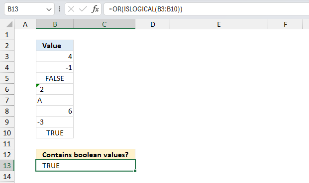
The MINA function evaluates TRUE to 1 and FALSE to 0 (zero), however, it can most often be useful to know if a given data set contains boolean values.

This example demonstrates how to find out if a cell range contains boolean or text values. Cell range B2:B10, in the image above, contains the following values:

Value
4
-1
FALSE
-2
A
6
-3
TRUE

Formula in cell B13:

This formula returns TRUE if the specified cell range contains at least one boolean or text value, this example shows that B3:B10 contains at least one boolean or text value. This formula can help you determine if you need to use the MIN function or the MINA function.

Explaining formula in cell B13

The Evaluate Formula tool is located on the Formulas tab in the Ribbon. It is a useful feature that allows you to step through and evaluate complex formulas to understand how the calculation is being performed and identify any errors or issues. The following steps shows these detailed evaluations for the formula above.

Step 1 - Identify boolean values

The ISLOGICAL function returns TRUE if value is boolean. A boolean value is either TRUE or FALSE.

Function syntax: ISLOGICAL(value)

ISLOGICAL(B3:B10)

becomes

ISLOGICAL({4;-1;FALSE;"-2";"A";6;"-3";TRUE})

and returns

{FALSE;FALSE;TRUE;FALSE;FALSE;FALSE;FALSE;TRUE}

Step 2 - Identify text values

The ISTEXT function returns TRUE if argument is text.

Function syntax: ISTEXT(value)

ISTEXT(B3:B10)

becomes

ISTEXT({4;-1;FALSE;"-2";"A";6;"-3";TRUE})

and returns

{FALSE;FALSE;FALSE;TRUE;TRUE;FALSE;TRUE;FALSE}

Step 3 - Apply OR logic

The OR function evaluates a logical expression in each argument and if at least one argument returns TRUE the OR function returns TRUE. If all arguments return FALSE the OR function also returns FALSE.

Function syntax: OR(logical1, [logical2])

OR(ISTEXT(B3:B10),ISLOGICAL(B3:B10))

becomes

OR({FALSE;FALSE;FALSE;TRUE;TRUE;FALSE;TRUE;FALSE},{FALSE;FALSE;TRUE;FALSE;FALSE;FALSE;FALSE;TRUE},)

and returns TRUE.

7. MINA function not working

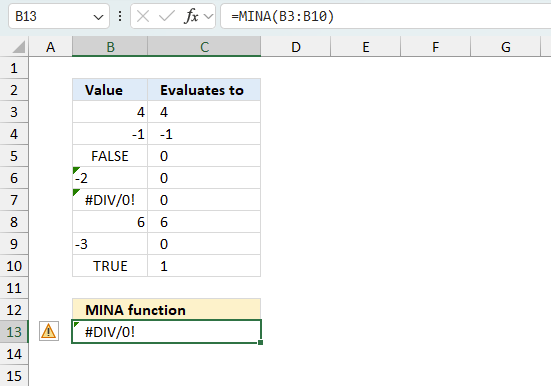
• MINA function returns 0 (zero) if argument has no values.
• Error values  in the source data cause the function to return an error.

Use the MIN function if you don't want to include logical values in the calculation.

7.1 Troubleshooting the error value

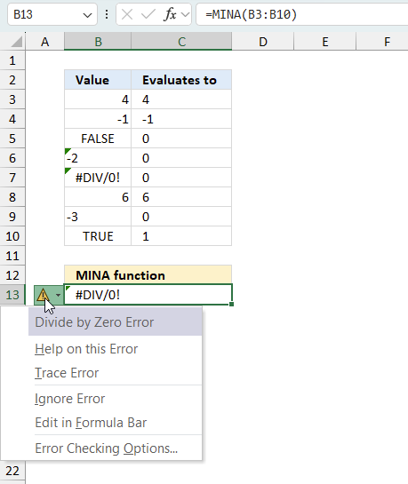
When you encounter an error value in a cell a warning symbol appears, displayed in the image above. Press with mouse on it to see a pop-up menu that lets you get more information about the error.

1. The first line describes the error if you press with left mouse button on it.
2. The second line opens a pane that explains the error in greater detail.
3. The third line takes you to the "Evaluate Formula" tool, a dialog box appears allowing you to examine the formula in greater detail.
4. This line lets you ignore the error value meaning the warning icon disappears, however, the error is still in the cell.
5. The fifth line lets you edit the formula in the Formula bar.
6. The sixth line opens the Excel settings so you can adjust the Error Checking Options.

Here are a few of the most common Excel errors you may encounter.

#NULL error - This error occurs most often if you by mistake use a space character in a formula where it shouldn't be. Excel interprets a space character as an intersection operator. If the ranges don't intersect an #NULL error is returned. The #NULL! error occurs when a formula attempts to calculate the intersection of two ranges that do not actually intersect. This can happen when the wrong range operator is used in the formula, or when the intersection operator (represented by a space character) is used between two ranges that do not overlap. To fix this error double check that the ranges referenced in the formula that use the intersection operator actually have cells in common.

#SPILL error - The #SPILL! error occurs only in version Excel 365 and is caused by a dynamic array being to large, meaning there are cells below and/or to the right that are not empty. This prevents the dynamic array formula expanding into new empty cells.

#DIV/0 error - This error happens if you try to divide a number by 0 (zero) or a value that equates to zero which is not possible mathematically.

#VALUE error - The #VALUE error occurs when a formula has a value that is of the wrong data type. Such as text where a number is expected or when dates are evaluated as text.

#REF error - The #REF error happens when a cell reference is invalid. This can happen if a cell is deleted that is referenced by a formula.

#NAME error - The #NAME error happens if you misspelled a function or a named range.

#NUM error - The #NUM error shows up when you try to use invalid numeric values in formulas, like square root of a negative number.

#N/A error - The #N/A error happens when a value is not available for a formula or found in a given cell range, for example in the VLOOKUP or MATCH functions.

#GETTING_DATA error - The #GETTING_DATA error shows while external sources are loading, this can indicate a delay in fetching the data or that the external source is unavailable right now.

7.2 The formula returns an unexpected value

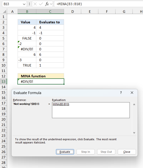
To understand why a formula returns an unexpected value we need to examine the calculations steps in detail. Luckily, Excel has a tool that is really handy in these situations. Here is how to troubleshoot a formula:

1. Select the cell containing the formula you want to examine in detail.
2. Go to tab “Formulas” on the ribbon.
3. Press with left mouse button on "Evaluate Formula" button. A dialog box appears.
   The formula appears in a white field inside the dialog box. Underlined expressions are calculations being processed in the next step. The italicized expression is the most recent result. The buttons at the bottom of the dialog box allows you to evaluate the formula in smaller calculations which you control.
4. Press with left mouse button on the "Evaluate" button located at the bottom of the dialog box to process the underlined expression.
5. Repeat pressing the "Evaluate" button until you have seen all calculations step by step. This allows you to examine the formula in greater detail and hopefully find the culprit.
6. Press "Close" button to dismiss the dialog box.

There is also another way to debug formulas using the function key F9. F9 is especially useful if you have a feeling that a specific part of the formula is the issue, this makes it faster than the "Evaluate Formula" tool since you don't need to go through all calculations to find the issue..

1. Enter Edit mode: Double-press with left mouse button on the cell or press F2 to enter Edit mode for the formula.
2. Select part of the formula: Highlight the specific part of the formula you want to evaluate. You can select and evaluate any part of the formula that could work as a standalone formula.
3. Press F9: This will calculate and display the result of just that selected portion.
4. Evaluate step-by-step: You can select and evaluate different parts of the formula to see intermediate results.
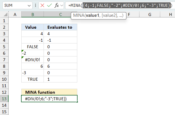
5. Check for errors: This allows you to pinpoint which part of a complex formula may be causing an error.

The image above shows cell reference B3:B10 converted to hard-coded value using the F9 key. The MINA function requires valid values which is not the case in this example. We have found what is wrong with the formula.

Tips!

• View actual values: Selecting a cell reference and pressing F9 will show the actual values in those cells.
• Exit safely: Press Esc to exit Edit mode without changing the formula. Don't press Enter, as that would replace the formula part with the calculated value.
• Full recalculation: Pressing F9 outside of Edit mode will recalculate all formulas in the workbook.

Remember to be careful not to accidentally overwrite parts of your formula when using F9. Always exit with Esc rather than Enter to preserve the original formula. However, if you make a mistake overwriting the formula it is not the end of the world. You can “undo” the action by pressing keyboard shortcut keys CTRL + z or pressing the “Undo” button

7.3 Other errors

Floating-point arithmetic may give inaccurate results in Excel - Article

Floating-point errors are usually very small, often beyond the 15th decimal place, and in most cases don't affect calculations significantly.

Functions in 'Statistical' category

The MINA function function is one of 73 functions in the 'Statistical' category.

Excel function categories

Excel categories

Leave a Comment