How to use the ISBLANK function
What is the ISBLANK function?
The ISBLANK function returns TRUE if the argument is an empty cell, returns FALSE if not.
Table of Contents
1. Introduction
What is a blank?
A blank refers to an empty cell, however, you can create a formula that returns nothing so it looks like the cell is empty when it is actually populated with a formula.
You can also populate a cell with a single or multiple blanks or spaces which are not visible. This makes the cell look empty but it is not.
What is an empty cell?
An empty cell is a cell that contains nothing at all.
What is a Boolean value?
A Boolean value in Excel is a value that can only be TRUE or FALSE. It represents binary logic and is the result of a logical expression using logical operators or a result of a few Excel functions that I'll discuss below.
Mastering Boolean logic and logical expressions is key to manipulating data and controlling workflow in Excel.
Other IS functions
| Excel Function | Description |
|---|---|
| ISBLANK(value) | Returns TRUE if the value is empty, FALSE otherwise |
| ISERR(value) | Returns TRUE if the value is any error value except #N/A, FALSE otherwise |
| ISERROR(value) | Returns TRUE if the value is any error value, FALSE otherwise |
| ISEVEN(value) | Returns TRUE if the value is an even number, FALSE for odd numbers |
| ISFORMULA(reference) | Returns TRUE if the cell contains a formula, FALSE otherwise |
| ISLOGICAL(value) | Returns TRUE if the value is a logical value (TRUE/FALSE), FALSE otherwise |
| ISNA(value) | Returns TRUE if the value is the #N/A error, FALSE otherwise |
| ISNONTEXT(value) | Returns TRUE if the value is not text, FALSE if it is text |
| ISNUMBER(value) | Returns TRUE if the value is a number, FALSE otherwise |
| ISODD(value) | Returns TRUE if the value is an odd number, FALSE for even numbers |
2. Syntax
ISBLANK(value)
| value | Required. The cell you want to check if empty. |
3. Example 1
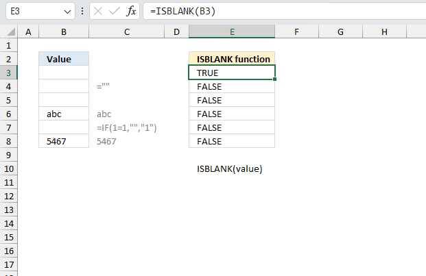
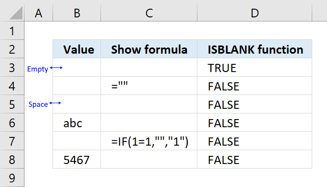
The image above shows different scenarios in column B and how the ISBLANK function handles them in column D. Column C contains what the cells in column B contain.
-
- Cell B3 is an empty blank cell, the ISBLANK function in cell D3 returns boolean value TRUE. Formula in cell D3:
=ISBLANK(B3)
- Cell B4 contains a formula which returns nothing specified by an equal sign and two double quotes. All formulas begin with an equal sign. Formula in cell D4:
=ISBLANK(B4)
Cell D4 returns FALSE, cell B4 is not blank.
- Cell B5 contains a space character which is of course not visible. Formula in cell D5:
=ISBLANK(B5)
Cell D5 returns FALSE, cell B4 is not empty blank.
- Cell B6 contains abc which is a text value. Formula in cell D6:
=ISBLANK(B6)
Cell D6 returns FALSE, cell B6 is not an empty blank cell.
- Cell B7 contains a formula. Formula in cell D7:
=ISBLANK(B6)
Cell D7 returns FALSE, cell B6 is not an empty blank cell.
- Cell B8 contains 5467 which is a numerical value. Formula in cell D8:
=ISBLANK(B6)
Cell D8 returns FALSE, cell B6 is not an empty blank cell.
- Cell B3 is an empty blank cell, the ISBLANK function in cell D3 returns boolean value TRUE. Formula in cell D3:
The ISBLANK function returns FALSE if a formula returns nothing, see picture above in cell B4 and B7. The ISBLANK function correctly identifies cells containing formulas as not empty even though they return nothing.
3.1 How to check if a formula returns nothing
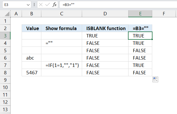
The ISBLANK function returns FALSE if a cell contains a fomrula theat evaluates to "" nothing. If this is not desired then use the equal sign to check if a formula returns nothing, use the following formula:
This returns TRUE if a formula returns nothing "" and FALSE if a formula returns a value.
4. Example 2
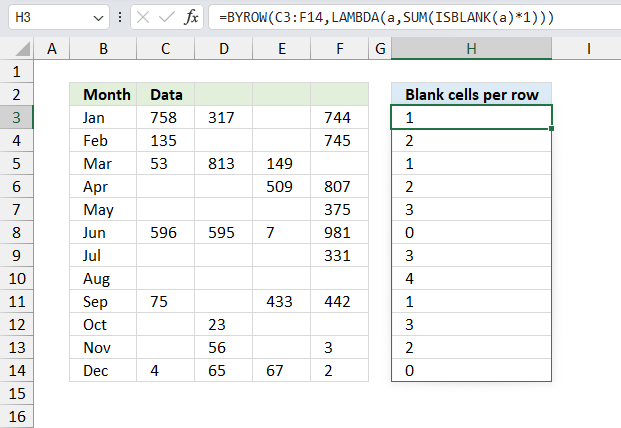
To complete a report on a scientific study you need to quantify the instances of missing data. How would you approach this task?
Cells B3:B14 contain months from January to December. Cell range C3:F14 contains numerical values. Formula in cell H3:
This is an Excel 365 dynamic array formula, it spills values automatically to adjacent cells as far as needed. The output array in cell range H3:H14 contains integers that represent the number of blank empty cells on the same row.
The first row has 1 empty blank cell, cell H3 returns 1 which corresponds the number of empty cells in C3:F3.
Explaining fomrula
Step 1 - Specify argument in BYROW function
The BYROW function puts values from an array into a LAMBDA function row-wise.
Function syntax: BYROW(array, lambda(array, calculation))
BYROW(C3:F14,....)
The first argument is a cell reference to C3:F14. The BYROW passes the values in C3:F14 row-wise to the LAMBDA function.
Step 2 - Specify argument in LAMBDA function
The LAMBDA function build custom functions without VBA, macros or javascript.
Function syntax: LAMBDA([parameter1, parameter2, …,] calculation)
BYROW(C3:F14,LAMBDA(a,...))
The argument in the LAMBDA function is a which is a variable. It will contain the values row by row.
Step 3 - Check if blank cells and convert boolean value to corresponding numerical value
We defined variable a in the step above, we can now use it to check if the values are empty blanks.
ISBLANK(a)*1 becomes ISBLANK({758,317,"",744})*1
becomes {FALSE, FALSE, TRUE, FALSE}*1
The SUM function ignores boolean values, we need to convert them to their numerical equivalents. This is easy simply multiply by 1.
{FALSE, FALSE, TRUE, FALSE}*1 returns {0,0,1,0}
Step 4 - Add numerical values and return a total by row
The SUM function allows you to add numerical values, the function returns the sum in the cell it is entered in. The SUM function is cleverly designed to ignore text and boolean values, adding only numbers.
Function syntax: SUM(number1, [number2], ...)
BYROW(C3:F14,LAMBDA(a,SUM(ISBLANK(a)*1)))
The sum function calculates a total per row, for example SUM(ISBLANK(a)*1) becomes
SUM({0,0,1,0}) and returns 1 which is the first value in the array. The BYROW function then reiterates these calculations using new values row-wise until all values have been processed.
It returns the following array: {1;2;1;2;3;0;3;4;1;3;2;0} displayed in cell range H3:H14 shown in the image above. The values correspond to the count of blank values in C3:F14 row by row.
5. Function not working
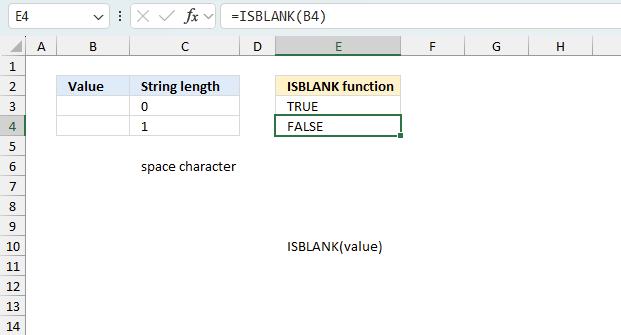
This example demonstrates two cells, B3 and B4, that seems to be empty, however cell B4 contains a space character.
Cell E3 and E4 contains the ISBLANK function and cell E3 returns TRUE meaning cell B3 is empty and cell E4 returns FALSE meaning cell B4 is not empty. This is hard tot tell, you can't see a space character. Ia m using the LEN function in cell C3 and C4 to show that cell B4 is not empty. 1 represents one character meaning cell B4 contains a character.
What is a space character?
A space character is a type of white-space character that represents the space between words or other characters in written text. It is a non-printing character, meaning it does not have a visible representation, but it occupies a position in the text and can affect the layout and formatting of the text. In computing and typing, the space character is typically created by pressing the space bar on a keyboard.
How to handle space characters in almost empty cells?
You can combine the TRIM function and the ISBLANK function to make the ISBLANK function return TRUE for cells containing a space character:
=ISBLANK(TRIM(B4))
It checks if a cell (B4 in this case) is blank after removing any leading or trailing spaces. This formula returns TRUE if cell B4 is empty or contains only spaces, and FALSE otherwise.
- TRIM(B4): The TRIM function removes any leading or trailing spaces from the text in cell B4. This ensures that the formula doesn't return a false negative if the cell contains only spaces.
- ISBLANK(...): The ISBLANK function checks if the result of the TRIM function is blank. If the cell is empty or contains only spaces (which were removed by the TRIM function), ISBLANK returns TRUE. Otherwise, it returns FALSE.
The ISBLANK function is one of the IS functions meaning they are somewhat different than other functions. The IS functions handle error values differently than other functions. When an IS function encounters an error value, such as #DIV/0! or #VALUE!, it returns FALSE.
In contrast, most other functions will propagate the error value and return the same error value. For example, if you try to use a mathematical function like SUM or AVERAGE on a range that contains an error value, the function will return the error value.
The IS functions, on the other hand, are designed to provide information about the input data and they will not propagate error values. Instead, they will return FALSE to indicate that the condition is not met.
7.1 Troubleshooting the error value
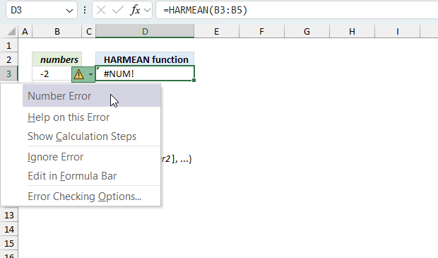
When you encounter an error value in a cell a warning symbol appears, displayed in the image above. Press with mouse on it to see a pop-up menu that lets you get more information about the error.
- The first line describes the error if you press with left mouse button on it.
- The second line opens a pane that explains the error in greater detail.
- The third line takes you to the "Evaluate Formula" tool, a dialog box appears allowing you to examine the formula in greater detail.
- This line lets you ignore the error value meaning the warning icon disappears, however, the error is still in the cell.
- The fifth line lets you edit the formula in the Formula bar.
- The sixth line opens the Excel settings so you can adjust the Error Checking Options.
Here are a few of the most common Excel errors you may encounter.
#NULL error - This error occurs most often if you by mistake use a space character in a formula where it shouldn't be. Excel interprets a space character as an intersection operator. If the ranges don't intersect an #NULL error is returned. The #NULL! error occurs when a formula attempts to calculate the intersection of two ranges that do not actually intersect. This can happen when the wrong range operator is used in the formula, or when the intersection operator (represented by a space character) is used between two ranges that do not overlap. To fix this error double check that the ranges referenced in the formula that use the intersection operator actually have cells in common.
#SPILL error - The #SPILL! error occurs only in version Excel 365 and is caused by a dynamic array being to large, meaning there are cells below and/or to the right that are not empty. This prevents the dynamic array formula expanding into new empty cells.
#DIV/0 error - This error happens if you try to divide a number by 0 (zero) or a value that equates to zero which is not possible mathematically.
#VALUE error - The #VALUE error occurs when a formula has a value that is of the wrong data type. Such as text where a number is expected or when dates are evaluated as text.
#REF error - The #REF error happens when a cell reference is invalid. This can happen if a cell is deleted that is referenced by a formula.
#NAME error - The #NAME error happens if you misspelled a function or a named range.
#NUM error - The #NUM error shows up when you try to use invalid numeric values in formulas, like square root of a negative number.
#N/A error - The #N/A error happens when a value is not available for a formula or found in a given cell range, for example in the VLOOKUP or MATCH functions.
#GETTING_DATA error - The #GETTING_DATA error shows while external sources are loading, this can indicate a delay in fetching the data or that the external source is unavailable right now.
7.2 The formula returns an unexpected value
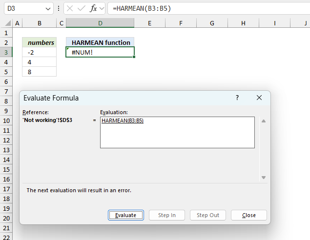
To understand why a formula returns an unexpected value we need to examine the calculations steps in detail. Luckily, Excel has a tool that Here is how to troubleshoot a formula:
- Select the cell containing the formula you want to examine in detail.
- Go to tab “Formulas” on the ribbon.
- Press with left mouse button on "Evaluate Formula" button. A dialog box appears.
The formula appears in a white field inside the dialog box. Underlined expressions are calculations being processed in the next step. The italicized expression is the most recent result. The buttons at the bottom of the dialog box allows you to evaluate the formula in smaller calculations which you control. - Press with left mouse button on the "Evaluate" button located at the bottom of the dialog box to process the underlined expression.
- Repeat pressing the "Evaluate" button until you have seen all calculations step by step. This allows you to examine the formula in greater detail and hopefully find the culprit.
- Press "Close" button to dismiss the dialog box.
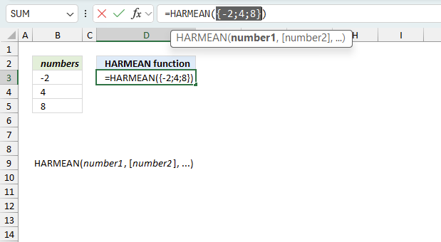
There is also another way to debug formulas using the function key F9. F9 is especially useful if you have a feeling that a specific part of the formula is the issue, this makes it faster than the "Evaluate Formula" tool since you don't need to go through all calculations to find the issue..
- Enter Edit mode: Double-press with left mouse button on the cell or press F2 to enter Edit mode for the formula.
- Select part of the formula: Highlight the specific part of the formula you want to evaluate. You can select and evaluate any part of the formula that could work as a standalone formula.
- Press F9: This will calculate and display the result of just that selected portion.
- Evaluate step-by-step: You can select and evaluate different parts of the formula to see intermediate results.
- Check for errors: This allows you to pinpoint which part of a complex formula may be causing an error.
The image above shows cell reference B3 converted to hard-coded value using the F9 key.
Tips!
- View actual values: Selecting a cell reference and pressing F9 will show the actual values in those cells.
- Exit safely: Press Esc to exit Edit mode without changing the formula. Don't press Enter, as that would replace the formula part with the calculated value.
- Full recalculation: Pressing F9 outside of Edit mode will recalculate all formulas in the workbook.
Remember to be careful not to accidentally overwrite parts of your formula when using F9. Always exit with Esc rather than Enter to preserve the original formula. However, if you make a mistake overwriting the formula it is not the end of the world. You can “undo” the action by pressing keyboard shortcut keys CTRL + z or pressing the “Undo” button
7.3 Other errors
Floating-point arithmetic may give inaccurate results in Excel - Article
Floating-point errors are usually very small, often beyond the 15th decimal place, and in most cases don't affect calculations significantly.
'ISBLANK' function examples
In this blog post I will demonstrate methods on how to find, select, and deleting blank cells and errors. Why […]
This article demonstrates Excel formulas that allows you to list unique distinct values from a single column and sort them […]
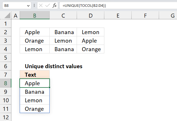
This article demonstrates ways to list unique distinct values in a cell range with multiple columns. The data is not […]
Functions in 'Information' category
The ISBLANK function function is one of 19 functions in the 'Information' category.


How to comment
How to add a formula to your comment
<code>Insert your formula here.</code>
Convert less than and larger than signs
Use html character entities instead of less than and larger than signs.
< becomes < and > becomes >
How to add VBA code to your comment
[vb 1="vbnet" language=","]
Put your VBA code here.
[/vb]
How to add a picture to your comment:
Upload picture to postimage.org or imgur
Paste image link to your comment.
Contact Oscar
You can contact me through this contact form