How to use the ROWS function

What is the ROWS function?

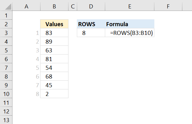
The ROWS function allows you to calculate the number of rows in a cell range.

The example above shows that cell range B3:B10 contains 8 rows.

1. Introduction

What is a cell reference?

A cell reference in Excel is a way to identify and refer to a specific cell or range of cells within a spreadsheet. Cell references are fundamental to Excel's functionality, allowing users to create dynamic, interconnected spreadsheets.

What is the cell reference structure?

It depends if the cell reference points to a single cell or a cell range containing multiple cells. A single cell reference typically consists of a column letter followed by a row number (e.g., A1, B2, C3).

A cell range reference points to multiple cells, for example: A1:B10. Note that the colon separates the first cell reference and the second cell reference. The first cell reference indicates the top-left cell in the specified cell range, while the second cell reference denotes the bottom-right cell in that same range. These two cell references determines the height in rows and width in columns, of the cell range. Cell range references are used in functions that perform calculations or operations on a group of cells, rather than just a single cell.

Both single cell and multi-cell references can also include sheet names for referencing cells in other worksheets. For example, Sheet!A1 or Sheet2!B2:B10. Note that Excel requires an exclamation mark between the sheet name and the cell reference. You can find the Sheet names your workbook contains, at the very bottom to the left. Single quotation marks are used if the worksheet name contains a space character, example: 'Budget 2027'!B3

What are the different cell reference types?

• Relative: The cell reference changes when the cell is copied or moved. For example: A1
• Absolute: The cell reference is fixed and doesn't change when copied. The dollar signs lets you specify which part of the cell reference you want to be abolute. For example: $A$1
• Mixed: One part fixed, one part relative. $A1 or A$1

When are cell references used?

In formulas to perform calculations using values from other cells. For data validation, conditional formatting, and other Excel features. To link data between different sheets or workbooks.

2. Syntax

ROWS(array)

array

Required. A cell range for which you want to calculate the number of rows.

Back to top

3. Example

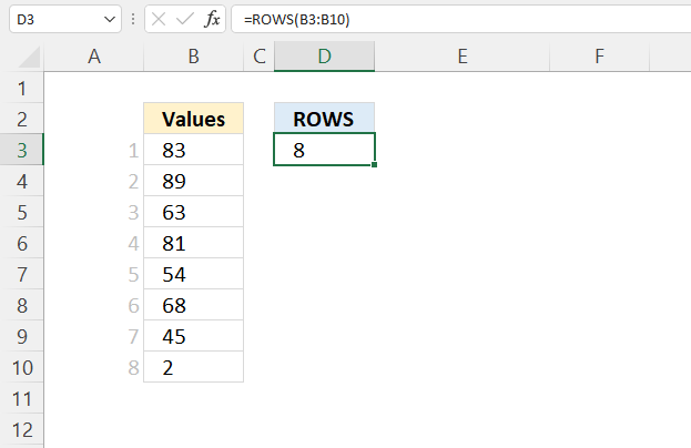
Formula in cell D3:

Back to top

4. Count rows in an array

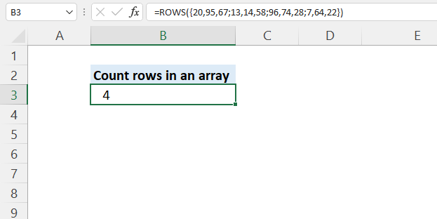
The ROWS function also calculates the number of rows in an array. This example demonstrates how to count rows in a hard coded array. An array is a collection of values that can be used in formulas and functions. It's a way to store and manipulate multiple values as a single unit.

A hard-coded array in Excel is an array that is explicitly defined within a formula using curly brackets {}. For example: {1, 2, 3, 4, 5}. This type of array is also known as a "constant array" or "literal array".

Formula in cell B3:

The array has four rows. The ; (semicolon) character is a row delimiting character in an array.

The delimiting characters in an array in Excel are:

• Commas (,) to separate values horizontally into columns. Using only column separated delimiters creates a one-dimensional array (e.g. {1, 2, 3, 4, 5}) The same thing applies if you only use row delimiters
• Semicolons (;) to separate values into rows in a two-dimensional array (e.g. {1, 2; 3, 4; 5, 6})
• Curly brackets {} to enclose the entire array

Back to top

5. Count rows based on a condition

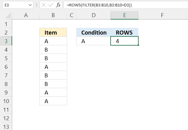
This formula is used to count the number of rows in a range that meet a specific condition. In other words, this formula is counting the number of cells in the range B3:B10 that have the same value as cell D3.

Formula in cell E3

Here is a breakdown of how it works:

• B3:B10 is the range of cells that we want to filter.
• D3 is the value that we want to match in the range.
• FILTER(B3:B10,B3:B10=D3) filters the range to only include cells that are equal to the value in cell D3.
• ROWS then counts the number of rows in the filtered range.

Explaining formula

Step 1 - Logical expression

The equal sign lets you compare value to value, it is also possible to compare a value to an array of values. The result is either TRUE or FALSE.

B3:B10=D3

becomes

{"A"; "B"; "B"; "A"; "B"; "B"; "A"; "A"}="A"

and returns

{TRUE; FALSE; FALSE; TRUE; FALSE; FALSE; TRUE; TRUE}.

Step 2 - Filter values based on a condition

The FILTER function gets values/rows based on a condition or criteria.
FILTER(array, include, [if_empty])

FILTER(B3:B10,B3:B10=D3)

becomes

FILTER({"A"; "B"; "B"; "A"; "B"; "B"; "A"; "A"}, {TRUE; FALSE; FALSE; TRUE; FALSE; FALSE; TRUE; TRUE})

and returns

{"A"; "A"; "A"; "A"}.

Step 3 - Count rows

ROWS(FILTER(B3:B10,B3:B10=D3))

becomes

ROWS({"A"; "A"; "A"; "A"})

and returns 4.

Back to top

6. Count rows based on a list

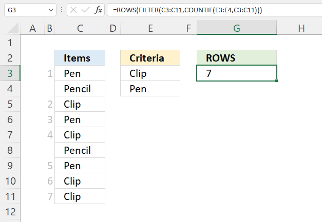
Formula in cell F3:

Explaining formula

Step 1 - Which values equal any item in the list

The COUNTIF function counts the number of cells that meet a given condition.
COUNTIF(range, criteria)

COUNTIF(E3:E4, C3:C11)

becomes

COUNTIF({"Clip"; "Pen"},{"Pen"; "Pencil"; "Clip"; "Pen"; "Clip"; "Pencil"; "Pen"; "Clip"; "Clip"})

and returns {1; 0; 1; 1; 1; 0; 1; 1; 1}.

Step 2 - Filter values based on array

The FILTER function gets values/rows based on a condition or criteria.
FILTER(array, include, [if_empty])

FILTER(C3:C11,COUNTIF(E3:E4,C3:C11))

becomes

FILTER({"Pen"; "Pencil"; "Clip"; "Pen"; "Clip"; "Pencil"; "Pen"; "Clip"; "Clip"}, {1; 0; 1; 1; 1; 0; 1; 1; 1})

and returns

{"Pen"; "Clip"; "Pen"; "Clip"; "Pen"; "Clip"; "Clip"}.

Step 3 - Count rows

ROWS(FILTER(C3:C11,COUNTIF(E3:E4,C3:C11)))

becomes

ROWS({"Pen"; "Clip"; "Pen"; "Clip"; "Pen"; "Clip"; "Clip"})

and returns 7.

Back to top

7. Count rows in a delimited string

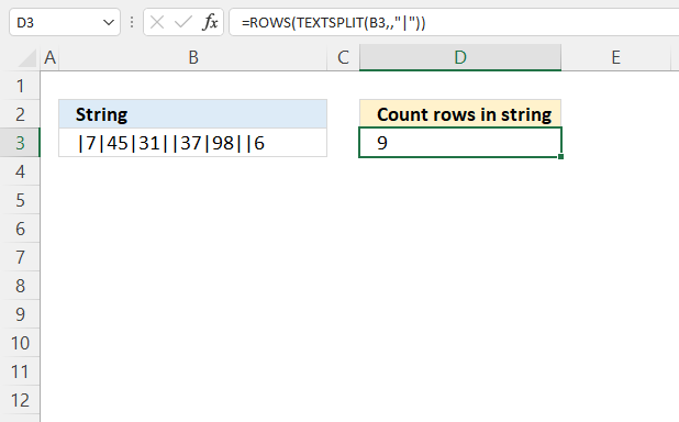
The formula in cell D3 counts delimited values in a string located in cell B3, you can use any character or string a s a delimiting character.

Excel 365 dynamic array formula in cell C3:

Explaining formula

Step 1 - Split string using a given delimiting character

The TEXTSPLIT function lets you split a string into an array across columns and rows based on delimiting characters.

TEXTSPLIT(B3,,";")

becomes

TEXTSPLIT("|7|45|31||37|98||6",,";")

and returns

{""; "7"; "45"; "31"; ""; "37"; "98"; ""; "6"}.

The semicolon is a delimiting character in arrays, however, they are determined by your regional settings. In other words, you may be using other delimtiing characters.

Step 2 - Count rows

ROWS(TEXTSPLIT(B3,,";"))

becomes

ROWS({""; "7"; "45"; "31"; ""; "37"; "98"; ""; "6"})

and returns 9. The values in the array are arranged vertically. An horizontal array would be using commas, like this: {"", "7", "45", "31", "", "37", "98", "", "6"}.

Back to top

8. Count rows in multiple cell ranges

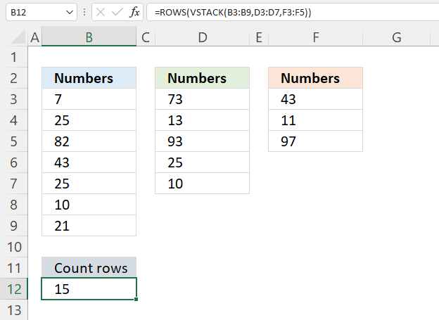
This example demonstrate how to count rows in three different sized cell ranges simultaneously and return total rows.

Formula in cell B12:

Explaining formula

Step 1 - Join arrays

The VSTACK function combines cell ranges or arrays, it joins data to the first blank cell at the bottom of a cell range or array.
VSTACK(array1,[array2],...)

VSTACK(B3:B9, D3:D7, F3:F5)

becomes

VSTACK({7; 25; 82; 43; 25; 10; 21},{73; 13; 93; 25; 10; 65; 91},{43; 11; 97; 61; 4; 45; 91})

and returns

{7; 25; 82; 43; 25; 10; 21; 73; 13; 93; 25; 10; 65; 91; 43; 11; 97; 61; 4; 45; 91}.

Step 2 - Calculate rows

ROWS(VSTACK(B3:B9,D3:D7,F3:F5))

becomes

ROWS({7; 25; 82; 43; 25; 10; 21; 73; 13; 93; 25; 10; 65; 91; 43; 11; 97; 61; 4; 45; 91})

and returns 15.

Back to top

9. Function not working

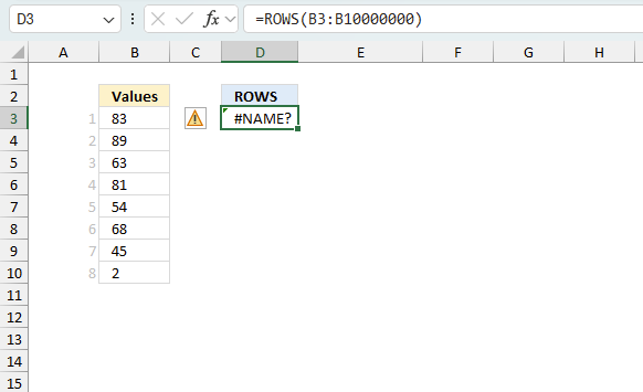
The ROWS function returns #NAME? error if you misspell the function name or use an invalid cell reference. The function will not propagate errors, meaning that if the input value contains an error (e.g., #VALUE!, #REF!), the function will not return the same error.

9.1 Troubleshooting the error value

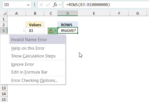
When you encounter an error value in a cell a warning symbol appears, displayed in the image above. Press with mouse on it to see a pop-up menu that lets you get more information about the error.

1. The first line describes the error if you press with left mouse button on it.
2. The second line opens a pane that explains the error in greater detail.
3. The third line takes you to the "Evaluate Formula" tool, a dialog box appears allowing you to examine the formula in greater detail.
4. This line lets you ignore the error value meaning the warning icon disappears, however, the error is still in the cell.
5. The fifth line lets you edit the formula in the Formula bar.
6. The sixth line opens the Excel settings so you can adjust the Error Checking Options.

Here are a few of the most common Excel errors you may encounter.

#NULL error - This error occurs most often if you by mistake use a space character in a formula where it shouldn't be. Excel interprets a space character as an intersection operator. If the ranges don't intersect an #NULL error is returned. The #NULL! error occurs when a formula attempts to calculate the intersection of two ranges that do not actually intersect. This can happen when the wrong range operator is used in the formula, or when the intersection operator (represented by a space character) is used between two ranges that do not overlap. To fix this error double check that the ranges referenced in the formula that use the intersection operator actually have cells in common.

#SPILL error - The #SPILL! error occurs only in version Excel 365 and is caused by a dynamic array being to large, meaning there are cells below and/or to the right that are not empty. This prevents the dynamic array formula expanding into new empty cells.

#DIV/0 error - This error happens if you try to divide a number by 0 (zero) or a value that equates to zero which is not possible mathematically.

#VALUE error - The #VALUE error occurs when a formula has a value that is of the wrong data type. Such as text where a number is expected or when dates are evaluated as text.

#REF error - The #REF error happens when a cell reference is invalid. This can happen if a cell is deleted that is referenced by a formula.

#NAME error - The #NAME error happens if you misspelled a function or a named range.

#NUM error - The #NUM error shows up when you try to use invalid numeric values in formulas, like square root of a negative number.

#N/A error - The #N/A error happens when a value is not available for a formula or found in a given cell range, for example in the VLOOKUP or MATCH functions.

#GETTING_DATA error - The #GETTING_DATA error shows while external sources are loading, this can indicate a delay in fetching the data or that the external source is unavailable right now.

9.2 The formula returns an unexpected value

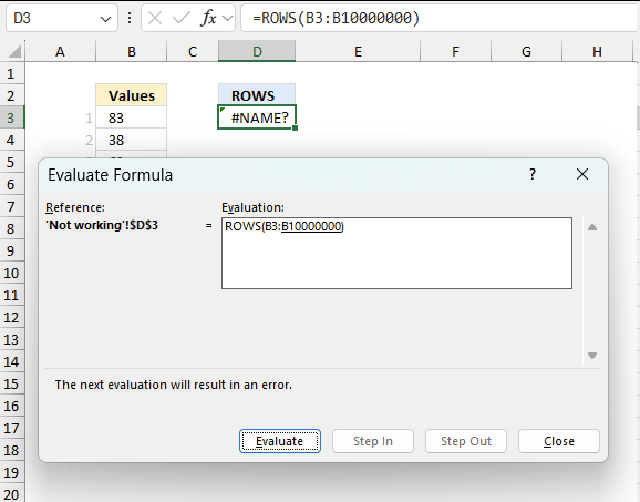
To understand why a formula returns an unexpected value we need to examine the calculations steps in detail. Luckily, Excel has a tool that is really handy in these situations. Here is how to troubleshoot a formula:

1. Select the cell containing the formula you want to examine in detail.
2. Go to tab “Formulas” on the ribbon.
3. Press with left mouse button on "Evaluate Formula" button. A dialog box appears.
   The formula appears in a white field inside the dialog box. Underlined expressions are calculations being processed in the next step. The italicized expression is the most recent result. The buttons at the bottom of the dialog box allows you to evaluate the formula in smaller calculations which you control.
4. Press with left mouse button on the "Evaluate" button located at the bottom of the dialog box to process the underlined expression.
5. Repeat pressing the "Evaluate" button until you have seen all calculations step by step. This allows you to examine the formula in greater detail and hopefully find the culprit.
6. Press "Close" button to dismiss the dialog box.

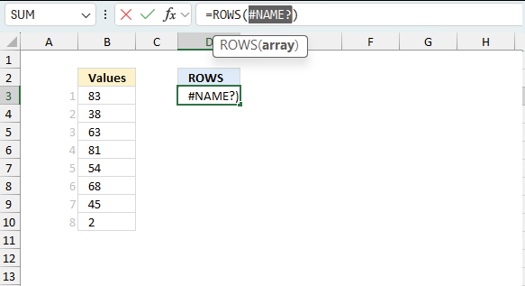
There is also another way to debug formulas using the function key F9. F9 is especially useful if you have a feeling that a specific part of the formula is the issue, this makes it faster than the "Evaluate Formula" tool since you don't need to go through all calculations to find the issue..

1. Enter Edit mode: Double-press with left mouse button on the cell or press F2 to enter Edit mode for the formula.
2. Select part of the formula: Highlight the specific part of the formula you want to evaluate. You can select and evaluate any part of the formula that could work as a standalone formula.
3. Press F9: This will calculate and display the result of just that selected portion.
4. Evaluate step-by-step: You can select and evaluate different parts of the formula to see intermediate results.
5. Check for errors: This allows you to pinpoint which part of a complex formula may be causing an error.

The image above shows the cell reference converted to hard-coded value using the F9 key. The ROWS function requires valid cell references which is not the case in this example. We have found what is wrong with the formula.

Tips!

• View actual values: Selecting a cell reference and pressing F9 will show the actual values in those cells.
• Exit safely: Press Esc to exit Edit mode without changing the formula. Don't press Enter, as that would replace the formula part with the calculated value.
• Full recalculation: Pressing F9 outside of Edit mode will recalculate all formulas in the workbook.

Remember to be careful not to accidentally overwrite parts of your formula when using F9. Always exit with Esc rather than Enter to preserve the original formula. However, if you make a mistake overwriting the formula it is not the end of the world. You can “undo” the action by pressing keyboard shortcut keys CTRL + z or pressing the “Undo” button

9.3 Other errors

Floating-point arithmetic may give inaccurate results in Excel - Article

Floating-point errors are usually very small, often beyond the 15th decimal place, and in most cases don't affect calculations significantly.

Useful links

ROWS function - Microsoft
ROWS Formula in Excel: Explained

'ROWS' function examples

Functions in 'Lookup and reference' category

The ROWS function function is one of 25 functions in the 'Lookup and reference' category.

Excel function categories

Excel categories

Leave a Comment