How to use the NETWORKDAYS function

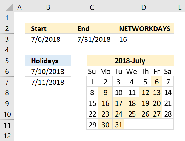
The NETWORKDAYS function returns the number of working days between two dates, excluding weekends. It also allows you to ignore a list of holiday dates that you can specify.

Formula in cell D3:

1. Introduction

What is the difference between the NETWORKDAYS.INTL function and the NETWORKDAYS function?

The NETWORKDAYS.INTL function lets you use custom weekend parameters. Actually they don't have to be a week end day, it can be a weekday also. This makes it really versatile for all sorts of calculations like how many mondays are there between a given start and end date.

Related functions

Excel Function	Description
NETWORKDAYS.INTL(start_date, end_date, weekend)	Returns the number of workdays between two dates, excluding custom weekend parameters
NETWORKDAYS(start_date, end_date)	Returns the number of workdays between two dates, excluding weekends
WORKDAY(start_date, days)	Returns a date adjusted by a number of workdays, excluding weekends
DATEDIF(start_date, end_date, unit)	Calculates the time between two dates in specified units like years, months, days
DAYS(end_date, start_date)	Returns the number of days between two specified dates

2. Syntax

NETWORKDAYS(start_date, end_date, [holidays])

3. Arguments

start_date	Required. The start date you want to use in the function.
end_date	Required. The end date you want to use.
[holidays]	Optional. Excludes this list of dates from being counted.

4. Example

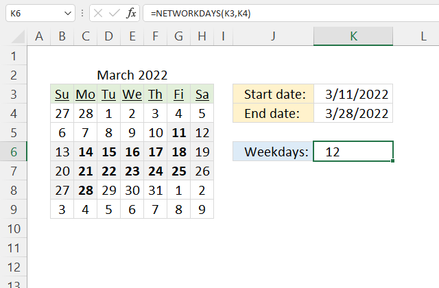
The formula in cell K6 counts weekdays (Monday to Friday) between two dates.

Formula in cell K6:

4.1 Explaining formula

Step 1 - NETWORKDAYS function

The NETWORKDAYS function returns the number of working days between two dates, excluding weekends. It also allows you to ignore a list of holiday dates that you can specify.

NETWORKDAYS(start_date, end_date, [holidays])

Step 2 - Populate arguments

The NETWORKDAYS function has three arguments, the third is optional.

start_date - K3

end_date - K4

[holidays] - Not used here

Step 3 - Evaluate NETWORKDAYS function

NETWORKDAYS(K3, K4)

becomes

NETWORKDAYS(44631, 44648)

and returns 12.

Back to top

5. Create a list of weekdays only

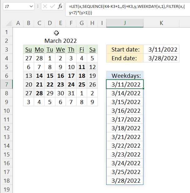
This example demonstrates how to extract a list of weekdays (Monday to Friday) or networking days. The formula in cell J7 uses the two dates specified in cells K3 and K4 to create a list of weekdays.

Excel 365 formula:

Explaining formula

This formula is a dynamic array formula and works only in Excel 365, it is entered as a regular formula

Step 1 - Calculate days between dates and add one

The minus and plus signs let you perform arithmetic operations in an Excel formula.

K4-K3+1

becomes

44648-44631+1

equals 18.

Step 2 - Create a sequence of numbers from 0 (zero) to 18

The SEQUENCE function creates a list of sequential numbers to a cell range or array. It is located in the Math and trigonometry category and is only available to Excel 365 subscribers.

SEQUENCE(rows, [columns], [start], [step])

SEQUENCE(K4-K3+1,,0)

becomes

SEQUENCE(18,,0)

and returns

{0; 1; 2; 3; 4; 5; 6; 7; 8; 9; 10; 11; 12; 13; 14; 15; 16; 17}.

Step 3 - Add start date to sequence of numbers

SEQUENCE(K4-K3+1,,0)+K3

becomes

{0; 1; 2; 3; 4; 5; 6; 7; 8; 9; 10; 11; 12; 13; 14; 15; 16; 17} + 44631

and returns

{44631; 44632; 44633; 44634; 44635; 44636; 44637; 44638; 44639; 44640; 44641; 44642; 44643; 44644; 44645; 44646; 44647; 44648}.

Step 4 - Calculate WEEKDAY number

WEEKDAY(SEQUENCE(K4-K3+1,,0)+K3,1)

becomes

WEEKDAY({44631; 44632; 44633; 44634; 44635; 44636; 44637; 44638; 44639; 44640; 44641; 44642; 44643; 44644; 44645; 44646; 44647; 44648},1)

and returns

{6; 7; 1; 2; 3; 4; 5; 6; 7; 1; 2; 3; 4; 5; 6; 7; 1; 2}.

Step 5 - Check if weekday number is smaller than 7

Seven is the last weekday in a week and it represents Saturday if the second argument is one. The smaller than character lets you compare values, the result is a boolean value TRUE or FALSE.

WEEKDAY(SEQUENCE(K4-K3+1,,0)+K3,1)<7

becomes

{6; 7; 1; 2; 3; 4; 5; 6; 7; 1; 2; 3; 4; 5; 6; 7; 1; 2}<7

and returns

{TRUE; FALSE; TRUE; TRUE; TRUE; TRUE; TRUE; TRUE; FALSE; TRUE; TRUE; TRUE; TRUE; TRUE; TRUE; FALSE; TRUE; TRUE}.

Step 6 - Check if weekday numbers are larger than one

One represents Sunday and we want to identify dates thare equal to Monday to Friday, in other words, networkingdays.

WEEKDAY(SEQUENCE(K4-K3+1,,0)+K3,1)>1

becomes

{6; 7; 1; 2; 3; 4; 5; 6; 7; 1; 2; 3; 4; 5; 6; 7; 1; 2}>1

and returns

{TRUE; TRUE; FALSE; TRUE; TRUE; TRUE; TRUE; TRUE; TRUE; FALSE; TRUE; TRUE; TRUE; TRUE; TRUE; TRUE; FALSE; TRUE}.

Step 7 - Multiply arrays

Both values on the same position in the arrays must return TRUE meaning we need to perform AND-logic. The asterisk lets us multiply values in an Excel formula.

TRUE * TRUE = 1
TRUE * FALSE = 0 (zero)
FALSE * FALSE = 0 (zero)

Boolean values have numerical equivalents, TRUE is equal to 1 and FALSE is equal to 0 (zero).

(WEEKDAY(SEQUENCE(K4-K3+1,,0)+K3,1)<7)*(WEEKDAY(SEQUENCE(K4-K3+1,,0)+K3,1)>1)

becomes

{TRUE; FALSE; TRUE; TRUE; TRUE; TRUE; TRUE; TRUE; FALSE; TRUE; TRUE; TRUE; TRUE; TRUE; TRUE; FALSE; TRUE; TRUE} * {TRUE; TRUE; FALSE; TRUE; TRUE; TRUE; TRUE; TRUE; TRUE; FALSE; TRUE; TRUE; TRUE; TRUE; TRUE; TRUE; FALSE; TRUE}

and returns

{1; 0; 0; 1; 1; 1; 1; 1; 0; 0; 1; 1; 1; 1; 1; 0; 0; 1}.

Step 8 - Filter dates based on conditions

The FILTER function is a new function available to Excel 365 subscribers. It lets you extract values based on a condition or criteria.

FILTER(array, include, [if_empty])

FILTER(SEQUENCE(K4-K3+1,,0)+K3,(WEEKDAY(SEQUENCE(K4-K3+1,,0)+K3,1)<7)*(WEEKDAY(SEQUENCE(K4-K3+1,,0)+K3,1)>1))

becomes

FILTER({44631; 44632; 44633; 44634; 44635; 44636; 44637; 44638; 44639; 44640; 44641; 44642; 44643; 44644; 44645; 44646; 44647; 44648},{1; 0; 0; 1; 1; 1; 1; 1; 0; 0; 1; 1; 1; 1; 1; 0; 0; 1})

and returns

{44631; 44634; 44635; 44636; 44637; 44638; 44641; 44642; 44643; 44644; 44645; 44648}.

Step 9 - Shorten formula

The LET function allows you to name intermediate calculation results which can shorten formulas considerably and improve performance.

LET(name1, name_value1, calculation_or_name2, [name_value2, calculation_or_name3...])

x - SEQUENCE(K4-K3+1, , 0)+K3
y - WEEKDAY(x, 1)

LET(x, SEQUENCE(K4-K3+1, , 0)+K3, y, WEEKDAY(x, 1), COUNT(FILTER(x, (y<7)*(y>1))))

Back to top

6. Count weekdays in a month

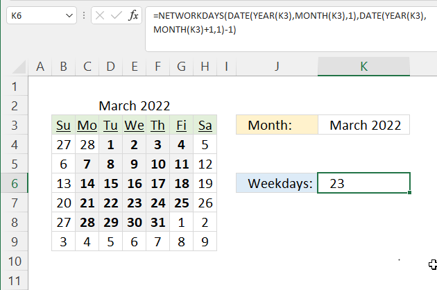
Formula in cell K6:

Explaining formula

Steps 1 to 3 calculate the first date of the specified month in cell K3. Steps 4 to 6 calculate the last date in the specified month.

Step 1 - Calculate year based on date

The YEAR function returns a number representing the year from a given date.

YEAR(date)

YEAR(K3)

becomes

YEAR(44631)

and returns 2022.

Step 2 - Calculate month based on date

The MONTH function returns a number representing the month from a given date.

MONTH(date)

MONTH(K3)

becomes

MONTH(44631)

and returns 3.

Step 3 - Calculate first date based on year and month

The DATE function returns an Excel date based on a year, month, and day number.

DATE(year, month, day)

DATE(YEAR(K3), MONTH(K3), 1)

becomes

DATE(2022, 3, 1)

and returns 44621. (3/1/2022)

Step 4 - Calculate year based on the date

YEAR(K3)

becomes

YEAR(44631)

and returns 2022.

Step 5 - Calculate year based on month

MONTH(K3)+1

becomes

MONTH(44631)+1

and returns 4.

Step 6 - Calculate the last date based on year and month

DATE(YEAR(K3),MONTH(K3)+1,1)-1

becomes

DATE(2022, 4, 1)-1

becomes

44652-1

and returns 44651. (3/31/2022)

Step 7 - Calculate the number of days between two dates

NETWORKDAYS(DATE(YEAR(K3),MONTH(K3),1),DATE(YEAR(K3),MONTH(K3)+1,1)-1)

becomes

NETWORKDAYS(44621, 44651)

and returns 23.

7. Holidays

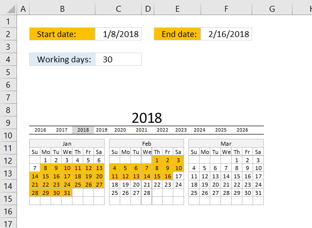
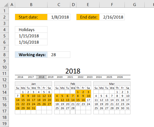
Excel contains a great function that easily counts the number of workdays between two dates, it even allows you to specify holidays that are not counted.

Formula in cell C4:

The image above shows two dates in cell range B5:B6 that acts as holidays in this example.

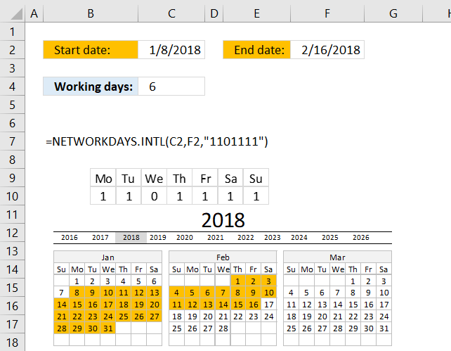
Formula in cell C8:

NETWORKDAYS.INTL function is available for Excel 2010 and later versions, it allows you to use custom weekends meaning if you want only Sundays to be weekend you can do that.

The string "1101111" means that all days except Wednesdays are weekends (isn't that great?) in the formula above, see row 9 and 10 above.

Back to top

8. Function not working

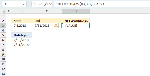
The NETWORKDAYS function returns

• #VALUE! error if you use an invalid Excel date.
• #NAME? error if you misspell the function name.
• propagates errors, meaning that if the input contains an error (e.g., #VALUE!, #REF!), the function will return the same error.

8.1 Troubleshooting the error value

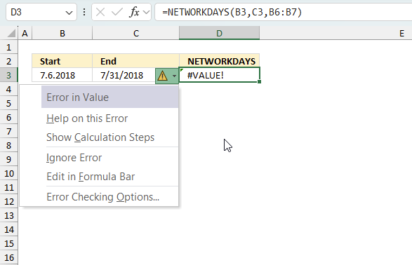
When you encounter an error value in a cell a warning symbol appears, displayed in the image above. Press with mouse on it to see a pop-up menu that lets you get more information about the error.

1. The first line describes the error if you press with left mouse button on it.
2. The second line opens a pane that explains the error in greater detail.
3. The third line takes you to the "Evaluate Formula" tool, a dialog box appears allowing you to examine the formula in greater detail.
4. This line lets you ignore the error value meaning the warning icon disappears, however, the error is still in the cell.
5. The fifth line lets you edit the formula in the Formula bar.
6. The sixth line opens the Excel settings so you can adjust the Error Checking Options.

Here are a few of the most common Excel errors you may encounter.

#NULL error - This error occurs most often if you by mistake use a space character in a formula where it shouldn't be. Excel interprets a space character as an intersection operator. If the ranges don't intersect an #NULL error is returned. The #NULL! error occurs when a formula attempts to calculate the intersection of two ranges that do not actually intersect. This can happen when the wrong range operator is used in the formula, or when the intersection operator (represented by a space character) is used between two ranges that do not overlap. To fix this error double check that the ranges referenced in the formula that use the intersection operator actually have cells in common.

#SPILL error - The #SPILL! error occurs only in version Excel 365 and is caused by a dynamic array being to large, meaning there are cells below and/or to the right that are not empty. This prevents the dynamic array formula expanding into new empty cells.

#DIV/0 error - This error happens if you try to divide a number by 0 (zero) or a value that equates to zero which is not possible mathematically.

#VALUE error - The #VALUE error occurs when a formula has a value that is of the wrong data type. Such as text where a number is expected or when dates are evaluated as text.

#REF error - The #REF error happens when a cell reference is invalid. This can happen if a cell is deleted that is referenced by a formula.

#NAME error - The #NAME error happens if you misspelled a function or a named range.

#NUM error - The #NUM error shows up when you try to use invalid numeric values in formulas, like square root of a negative number.

#N/A error - The #N/A error happens when a value is not available for a formula or found in a given cell range, for example in the VLOOKUP or MATCH functions.

#GETTING_DATA error - The #GETTING_DATA error shows while external sources are loading, this can indicate a delay in fetching the data or that the external source is unavailable right now.

8.2 The formula returns an unexpected value

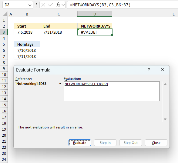
To understand why a formula returns an unexpected value we need to examine the calculations steps in detail. Luckily, Excel has a tool that is really handy in these situations. Here is how to troubleshoot a formula:

1. Select the cell containing the formula you want to examine in detail.
2. Go to tab “Formulas” on the ribbon.
3. Press with left mouse button on "Evaluate Formula" button. A dialog box appears.
   The formula appears in a white field inside the dialog box. Underlined expressions are calculations being processed in the next step. The italicized expression is the most recent result. The buttons at the bottom of the dialog box allows you to evaluate the formula in smaller calculations which you control.
4. Press with left mouse button on the "Evaluate" button located at the bottom of the dialog box to process the underlined expression.
5. Repeat pressing the "Evaluate" button until you have seen all calculations step by step. This allows you to examine the formula in greater detail and hopefully find the culprit.
6. Press "Close" button to dismiss the dialog box.

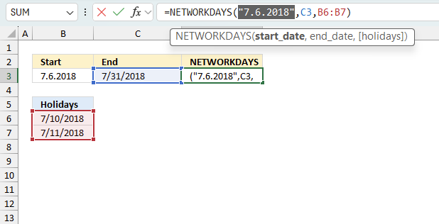
There is also another way to debug formulas using the function key F9. F9 is especially useful if you have a feeling that a specific part of the formula is the issue, this makes it faster than the "Evaluate Formula" tool since you don't need to go through all calculations to find the issue..

1. Enter Edit mode: Double-press with left mouse button on the cell or press F2 to enter Edit mode for the formula.
2. Select part of the formula: Highlight the specific part of the formula you want to evaluate. You can select and evaluate any part of the formula that could work as a standalone formula.
3. Press F9: This will calculate and display the result of just that selected portion.
4. Evaluate step-by-step: You can select and evaluate different parts of the formula to see intermediate results.
5. Check for errors: This allows you to pinpoint which part of a complex formula may be causing an error.

The image above shows cell reference B3 converted to hard-coded value using the F9 key. The NETWORKDAYS function requires valid Excel dates which is not the case in this example. We have found what is wrong with the formula.

Tips!

• View actual values: Selecting a cell reference and pressing F9 will show the actual values in those cells.
• Exit safely: Press Esc to exit Edit mode without changing the formula. Don't press Enter, as that would replace the formula part with the calculated value.
• Full recalculation: Pressing F9 outside of Edit mode will recalculate all formulas in the workbook.

Remember to be careful not to accidentally overwrite parts of your formula when using F9. Always exit with Esc rather than Enter to preserve the original formula. However, if you make a mistake overwriting the formula it is not the end of the world. You can “undo” the action by pressing keyboard shortcut keys CTRL + z or pressing the “Undo” button

8.3 Other errors

Floating-point arithmetic may give inaccurate results in Excel - Article

Floating-point errors are usually very small, often beyond the 15th decimal place, and in most cases don't affect calculations significantly.

'NETWORKDAYS' function examples

Functions in 'Date and Time' category

The NETWORKDAYS function function is one of 22 functions in the 'Date and Time' category.

Excel function categories

Excel categories

Comments (1)