Time sheet for work

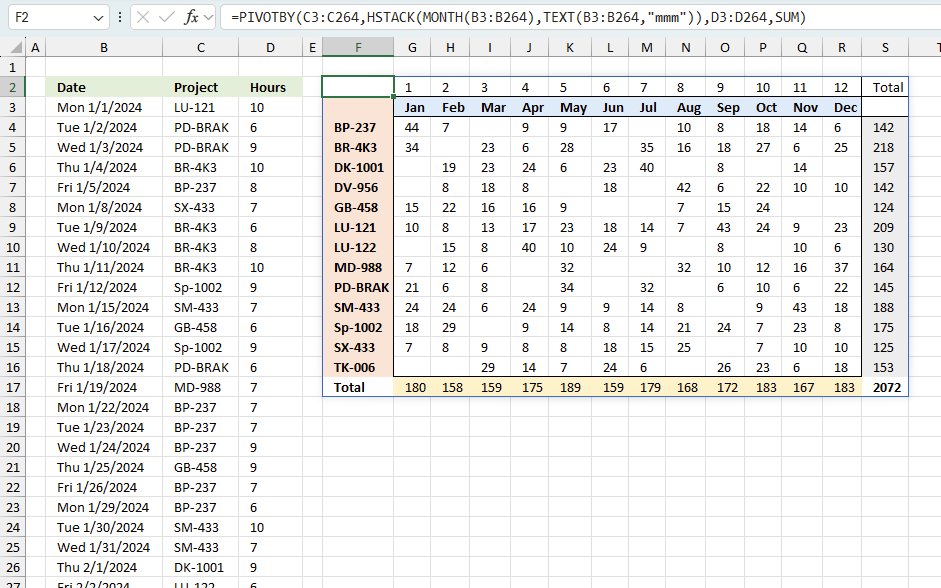
The image above shows how to summarize work hours using the new GROUPBY function in Excel 365. This is demonstrated in section 2 below.

1. Time sheet for work - alternative 1

I have built a sheet to track time at work. It is very simple, there are 13 sheets, one for each month and a worksheet containing totals for each project.

The above picture shows you January 2017, simply enter the project name in column A and the hours in cell range B5:AF32. Row 4 contains dates for January, row 3 the weekdays, and row 2 the week numbers. Saturday and Sundays are colored grey.

1.1. How it works

The Summary sheet, see picture above, contains all projects entered in all month sheets and a total, both for the month and project. A quite large array formula extracts all project names in column B, you don't need to do that manually.

A simple SUMIF function sums the values from each monthly sheet, excel takes care of that too. There is no VBA in this workbook, you can find the get link at the end of this article.

If you change the year on sheet "Summary" you will notice that the monthly sheets change accordingly, you don't need to change weekdays, week number, or color weekends on each sheet, Excel will do it for you.

Any suggestions for improvement?

Back to top

1.2. How I built this time tracker

The workbook has a summary sheet and sheets for each month in a year. The summary sheet allows you to enter the year in cell H1, I also changed the font size for that cell.

Back to top

1.2.1 Building monthly sheets

The first monthly sheet is January, this sheet will be the template for the remaining months. This means I will copy this sheet and change the date for each sheet.

Cell D1 contains this formula: =Summary!H1
This lets you change the year on the summary sheet and all other monthly sheets will be instantly updated.

Formula in cell I1: =DATE(D1,1,1)
Select cell I1 and press CTRL + 1 to open the formatting cells dialog box. Change formatting category to "Custom".

Change Type to MMMM;@
If this is not working you need to find out your regional settings in Windows and change MMMM accordingly. This web page from Microsoft explains how to use the formatting dialog box.

This is what cell I1 now looks like:

Time to add dates,type 1 to 31 in cell range B4:AH4. I also change the cell width to 21 pixels. Type "Project" in cell A4, cells below contains project names.

Add text "Total:" to cell AG4 and use this formula in cell AG5:=SUM(B5:AF5)
Copy cell AG5 and paste to cell range AG6:AG32. See picture below.

Add text "Total:" to cell A33 and use this formula in cell B33:=SUM(B5:B32)
Copy cell A33 and paste to cell range B33:AF33. See picture above.

To make this sheet easier to read I want the row above dates to contain the abbreviation of days of the week. I am using this formula in cell B3:

I also want the row above days of the week to contain the week number. Formula in cell B2:

But I only want that number above a date when a new week starts.

Formula in cell C2:

Copy cell C2 and paste to D2:AF2. See pic below.

Back to top

1.2.2 Highlight weekends

The following conditional formatting formula highlights weekends gray:

(WEEKDAY(B$4,2)>5)*(MONTH(B$4)=MONTH($B$4))

1. Select cell range B4:AF32
2. Go to tab Home on the ribbon
3. Press with left mouse button on "Conditional Formatting" button and then press with left mouse button on "New Rule.."
4. Press with left mouse button on "Use a formula to determine which cells to format"
5. Paste above formula to field "Format values where this formula is true:"
   
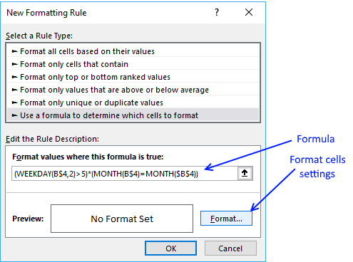
6. Press with left mouse button on "Format" button
7. Go to tab "Fill"
8. Pick a color
   
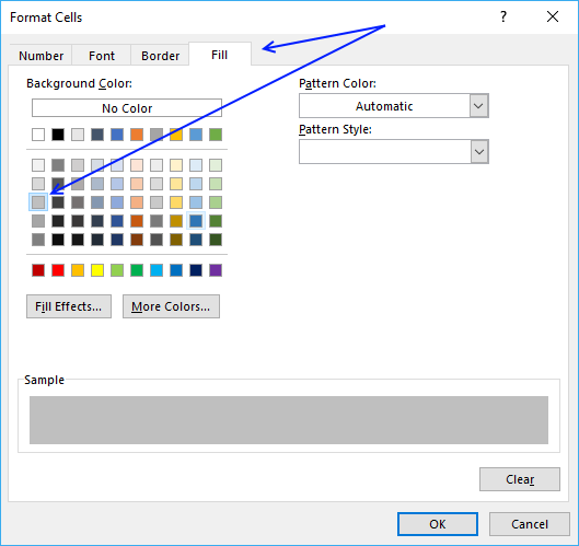
9. Press with left mouse button on OK button

Worksheet "January" now looks like this:

The conditional formatting changes depending on what month and year it is, this is not something you have to manually do.

Back to top

1.2.3 Grid pattern - Conditional Formatting

The next thing is the grid pattern, here is the conditional formatting formula:

=IF($AI$3="Off",,MONTH(B$4)=MONTH($B$4))

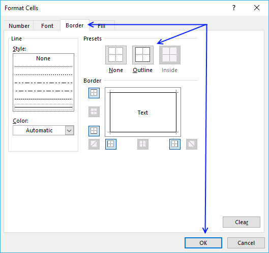
To build formatting formula, repeat above steps 1 to 8 except instead of picking a color, go to tab "Border" and press with left mouse button on "Outline, then press with left mouse button on the OK button. See the picture below.

Back to top

1.2.4 Create remaining months

Worksheet January is now ready, time to copy the worksheet and create worksheets for the remaining months.

1. Press with right mouse button on on the worksheet "January".
2. Press with left mouse button on "Move or Copy...".
3. Select "move to end" and "Create a copy".
4. Press with left mouse button on the OK button.

Repeat above steps until you have a worksheet for each month in a year.

1. Rename the sheet after January to February
2. Change formula in cell I1 to =DATE(D1,2,1)
   Note that February is the second month in a year and the second argument in the formula is then 2.

Repeat steps 1 and 2 above for all remaining worksheets.

Back to top

1.2.5 Totals worksheet

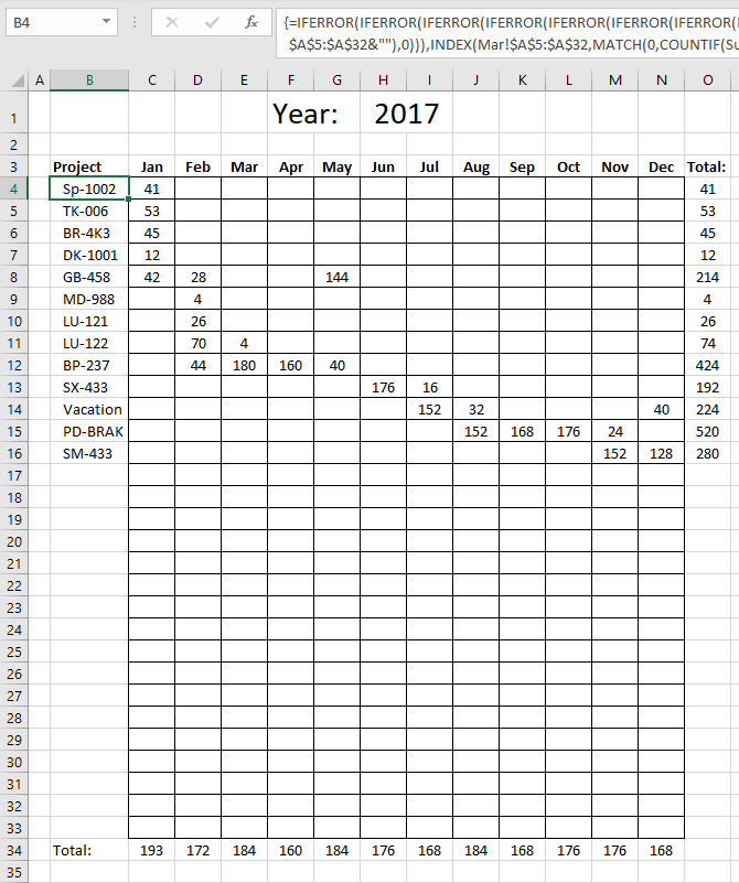
The following formulas extracts the project names from worksheet Jan to Dec, however, only one instance per name meaning duplicate values are ignored.

The first formula works only in Excel 365, it uses two Excel functions and a 3D cell reference that points to A5:A32 across all worksheets between Jan to Dec. The  formula below the 365 dynamic array formula is for earlier Excel. It is mind blowing how much more efficient the new Excel 365 functions are.

Excel 365 dynamic array formula in cell B4:

Here is a quick break-down of the formula:

This Excel 365 formula uses two functions: UNIQUE and TOCOL.

1. TOCOL is a function that converts a 2D range into a 1D array. In this case, it's being used to convert the range Jan:Dec!A5:A32 into a single column array. The "1" at the end of the TOCOL function indicates that blank cells will be ignored.
2. UNIQUE is a function that returns a list of unique distinct values from a range or array. In this case, it's being used to return a list of unique distinct values from the array created by the TOCOL function.

The formula will return a list of unique values from the range A5:A32 across all worksheets named Jan through Dec.

Formula in cell B4, earlier Excel versions:

Explaining formula in cell B4

INDEX(Jan!$A$5:$A$32 , MATCH(0 , COUNTIF(Summary!$B$2:B3 , Jan!$A$5:$A$32&"") , 0))

Step 1 - Check previous values above the current cell

The COUNTIF function calculates the number of cells that is equal to a condition.

COUNTIF(range, criteria)

COUNTIF(Summary!$B$2:B3 , Jan!$A$5:$A$32&"")

becomes

COUNTIF({0;"Project"}, {"Sp-1002"; "TK-006"; "BR-4K3"; "DK-1001"; "GB-458"; ""; ""; ""; ""; ""; ""; ""; ""; ""; ""; ""; ""; ""; ""; ""; ""; ""; ""; ""; ""; ""; ""; ""})

and returns {0; 0; 0; 0; 0; 1; 1; 1; 1; 1; 1; 1; 1; 1; 1; 1; 1; 1; 1; 1; 1; 1; 1; 1; 1; 1; 1; 1}.

Note that the COUNTIF function also returns 1 for empty cells.

Step 2 - Find relative position of a not yet shown value

The MATCH function returns the relative position of an item in an array or cell reference that matches a specified value in a specific order.

MATCH(lookup_value, lookup_array, [match_type])

We are looking for values not yet displayted in cells above the current cell. 0 (zero) indicates it has not yet been shown.

MATCH(0 , COUNTIF(Summary!$B$2:B3 , Jan!$A$5:$A$32&"") , 0)

becomes

MATCH(0 , {0; 0; 0; 0; 0; 1; 1; 1; 1; 1; 1; 1; 1; 1; 1; 1; 1; 1; 1; 1; 1; 1; 1; 1; 1; 1; 1; 1} , 0)

and returns 1.

Step 3 - Return value

The INDEX function returns a value from a cell range, you specify which value based on a row and column number.

INDEX(array, [row_num], [column_num])

INDEX(Jan!$A$5:$A$32 , MATCH(0 , COUNTIF(Summary!$B$2:B3 , Jan!$A$5:$A$32&"") , 0))

becomes

INDEX(Jan!$A$5:$A$32, 1)

becomes

INDEX({"Sp-1002"; "TK-006"; "BR-4K3"; "DK-1001"; "GB-458"; ""; ""; ""; ""; ""; ""; ""; ""; ""; ""; ""; ""; ""; ""; ""; ""; ""; ""; ""; ""; ""; ""; ""}, 1)

and returns "Sp-1002" in cell B4.

Step 4 - Go to the next worksheet

The IFERROR function lets you use another formula when there are no more values to display. This behavior is called nested functions and is repeated to include all worksheets.

IFERROR(INDEX(Jan!$A$5:$A$32 , MATCH(0 , COUNTIF(Summary!$B$2:B3 , Jan!$A$5:$A$32&"") , 0)) , INDEX(Feb!$A$5:$A$32 , MATCH(0 , COUNTIF(Summary!$B$2:B3 , Feb!$A$5:$A$32&"") , 0)))

Back to top

Get the Excel file

Work-time-trackerv3.xlsx

2. Time sheet for work - Alternative 2

This worksheets lets you enter the date, project name, and the number of hours in columns B, C, and D respectively. The formula in cell F2 creates a pivot table based on the input values.

• Project names are displayed in F3:F16
• Months are shown in G3:R3
• The hours are aggregated and shown for each project based on the month
• Totals are displayed below and to the right of the numbers.
• A grand total is shown in cell S17.

Excel 365 dynamic array formula in cell F2:

Here is a break-down:

1. PIVOTBY(C3:C264, ... , D3:D264, SUM): This is the main function. It's summarizing data from columns C and D, from rows 3 to 264.
2. HSTACK(MONTH(B3:B264), TEXT(B3:B264,"mmm")): This part creates the categories for grouping the data.
   1. MONTH(B3:B264) extracts the month number (1-12) from dates in column B. This is included so the months get sorted from January to December.
   2. TEXT(B3:B264,"mmm") converts the dates to three-letter month abbreviations (e.g., Jan, Feb, Mar).
   3. HSTACK combines these two results into a single array.
3. SUM: This is the aggregation function, summing the values in column D for each group.

This formula groups data by both the month number and month name abbreviation from column B. For each project, it sums the corresponding values from column D. The results are organized based on the unique projects in column C. This creates a summary table showing totals for each month with both the month number and abbreviation as identifiers categorized by the values in column C.

Work time trackerv4.xlsx

Templates category

Monthly calendar template
Table of Contents Monthly calendar template Monthly calendar template 2 Calendar - monthly view - Excel 365 Calendar - monthly […]

Excel template: Getting Things Done [VBA]
In this article, I am going to demonstrate a simple workbook where you can create or delete projects and add […]

Highlight events in a yearly calendar
This article demonstrates how to highlight given date ranges in a yearly calendar, this calendar allows you to change the […]

Excel categories

Comments (10)