How to use the TEXTJOIN function
What is the TEXTJOIN function?
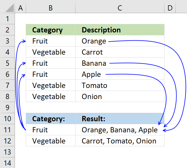
The TEXTJOIN function allows you to combine text strings from multiple cell ranges and also use delimiting characters if you want. Not only that, you can also use it in array formulas.
The TEXTJOIN function is a relatively new function introduced in Excel 2019, it is like the CONCATENATE function on steroids or what the CONCATENATE function should have been from the beginning.
What's on this page
- Syntax
- Arguments
- How to join cell values without a delimiting character
- How to concatenate cell values ignoring empty cells
- Concatenate values based on a condition
- User Defined Function alternative (VBA)
- VBA code
- Where do I put this code?
- How do I use it?
- UDF arguments
- UDF Syntax
- How to add row delimiting characters
- Get Excel File
- Workaround for the TEXTSPLIT function - LAMBDA function
- Function not working
TEXTJOIN alternatives for earlier Excel versions
- Concatenate cell values in a row into a single cell
- Concatenate cell values in a column into a single cell
- Concatenate a multi-column and multi-row cell range
- Create delimiting character
Concatenate unique distinct values
1. Syntax
TEXTJOIN(delimiter, ignore_empty, text1, [text2], ...)
2. Arguments
| delimiter | Required. The delimiting character or characters you want to use. |
| ignore_empty | Required. True lets you ignore empty cells in the third argument, False adds empty cells to the output. |
| text1 | Required. The cell range you want to concatenate. |
| [text2] | Optional. Up to 254 additional cell ranges. |
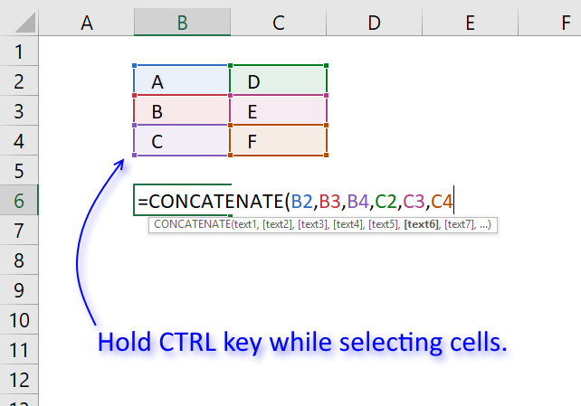
The similar CONCATENATE function forced you to select each cell in order to join text strings, see picture below. If you had to combine many many cells this function was not an option, you had to use a custom vba function.
You can use the TEXTJOIN function with a cell range or multiple cell ranges, this may save you a lot of time if you are working with many cells.
3. How to join cell values without a delimiting character
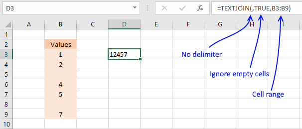
The first argument in the TEXTJOIN function is the delimiter, the example above shows you the result in cell C4 if you use no delimiting characters.
The second argument lets you choose between TRUE or FALSE, if TRUE it will ignore empty cells. The third argument is the cell range.
The following article shows you how to add unique distinct values to a cell using the TEXTJOIN function:
Recommended articles
This article demonstrates Excel formulas that extract unique distinct values from a cell range and concatenates the values using any […]
4. How to concatenate cell values ignoring empty cells
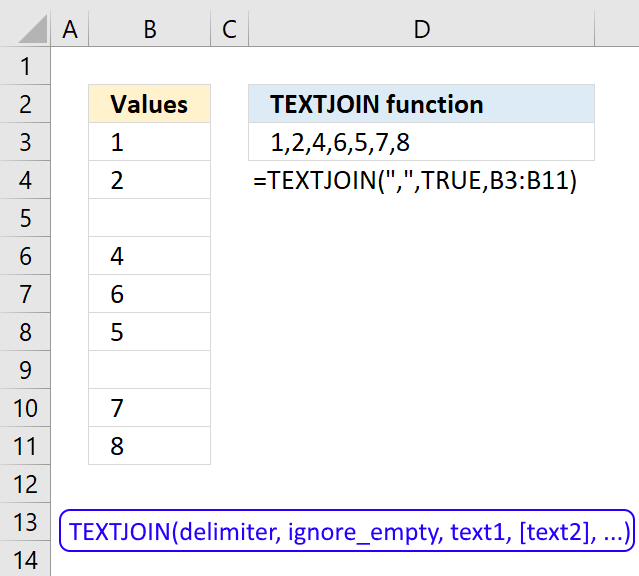
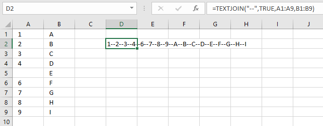
This picture shows you the TEXTJOIN function combining multiple cell ranges with a delimiting text string. It also ignores the empty cell A5. You can use up to 252 cell ranges.
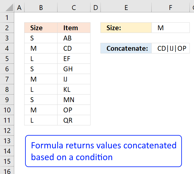
5. How to concatenate values based on a condition
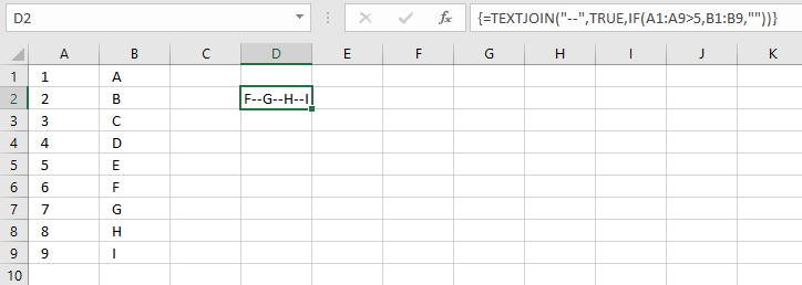
It is possible to use the TEXTJOIN function in an array formula, here is a simple demonstration. You can see that the third argument contains:
This IF function checks if the numbers in cell range A1:A9 are above 5 and if they are the corresponding value in cell range B1:B9 is returned.
Numbers 6,7,8 and 9 are larger than 5 so corresponding characters F, G, H, and I are combined using the delimiting characters "--".
5.1 Explaining formula
Step 1 - Logical expression
The larger than character is a logical operator that lets you check if a number is larger than another number, the result is a boolean value TRUE or FALSE.
A1:A9>5
returns {FALSE; ... ; TRUE}.
Step 2 - Evaluate IF function
The IF function returns one value if the logical test is TRUE and another value if the logical test is FALSE.
IF(logical_test, [value_if_true], [value_if_false])
IF(A1:A9>5,B1:B9,"")
returns {""; ""; ""; ""; ""; "F"; "G"; "H"; "I"}.
Step 3 - Join values
TEXTJOIN("--", TRUE, IF(A1:A9>5, B1:B9, ""))
returns "F--G--H--I".
This post demonstrates how to do a lookup and concatenate returning values:
Recommended articles
This article demonstrates how to find a value in a column and concatenate corresponding values on the same row. The […]
6. TEXTJOIN function VBA for previous Excel versions
The following user defined function (udf) allows you to combine text strings just like the TEXTJOIN function.
Why would you want to use this udf? TEXTJOIN function is only available in Excel 365, previous excel versions are missing this function.
6.1 VBA code
'Name User Defined Function, specify parameters and declare data types
Function TEXTJOIN(delimiter As String, ignore_empty As Boolean, ParamArray cell_ar() As Variant)

'For each statement, iterate through each cell range
For Each cellrng In cell_ar

'For each statement, iterate through each cell in cell range
For Each cell In cellrng

'If ... Then ... Else ... End If statement
'Check if parameter ignore_empty is equal to boolean value False
If ignore_empty = False Then

'Concatenate cell value and delimiter with variable result and save to result
result = result & cell & delimiter

'Go here if ignore_empty is not equal to False
Else

'Check if cell value is not equal to nothing
If cell <> "" Then

'Concatenate cell value and delimiter with variable result and save to result
result = result & cell & delimiter
End If
End If

'Continue with next cell value
Next cell

'Continue with next cell range
Next cellrng

'Remove last delimiter in variable result and return values to worksheet
TEXTJOIN = Left(result, Len(result) - Len(delimiter))
End Function
6.2 Where do I put this code?
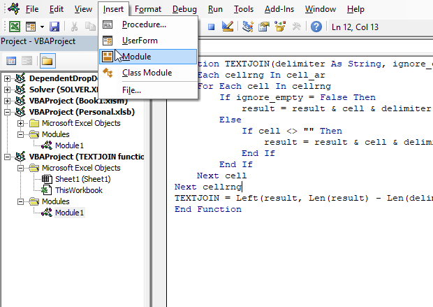
- Press Alt + F11 to open the Visual Basic Editor (VBE).
- Press with left mouse button on "Insert" on the menu.
- Press with left mouse button on "Module".
- Copy code above.
- Paste it to the code module.
- Exit VB Editor.
6.3 How do I use it?
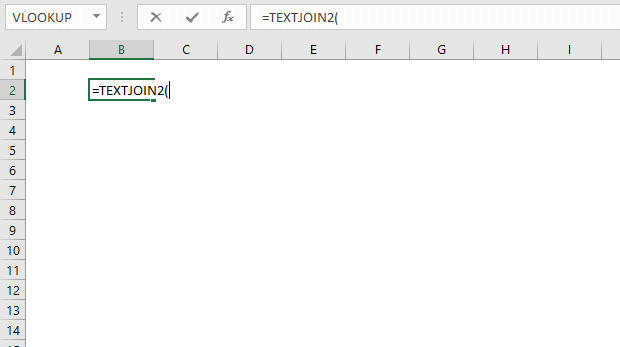
- Select a cell.
- Type Textjoin(
- Type your three arguments and ending parentheses.
- Press Enter.
6.4 UDF arguments
delimiter - A text string, if you want nothing type ""
ignore_empty - If TRUE it ignores empty cells
text1, text2, ... - A cell range or multiple cell ranges. Use a comma to separate them.
6.5 UDF Syntax
TEXTJOIN(delimiter, ignore_empty, [text1, text2, ...])
7. TEXTJOIN function - how to add row delimiting characters
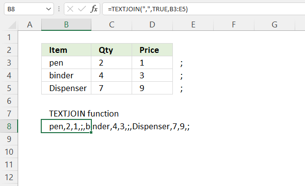
The TEXTSPLIT function allows you to split a string using both column and row delimiting characters, however, the TEXTJOIN function lets you only use a column delimiting character.
There is a workaround to add row delimiting characters, add your row delimiting character after the last cell on each row, see the image above cell range E3:E5.
You can now use the TEXTSPLIT function to split the string to create a 2D array, 2D array is an array with both columns and rows.
9. Workaround for the TEXTSPLIT function - LAMBDA function
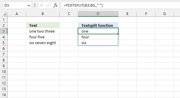
The TEXTSPLIT function splits a string into an array based on delimiting values.
Function syntax: TEXTSPLIT(Input_Text, col_delimiter, [row_delimiter], [Ignore_Empty])
The TEXTSPLIT function works only with single cells. If you try to use a cell range the TEXTSPLIT function returns only the first value in each cell. See the image above.
Formula in cell D3:
There is a workaround for this.
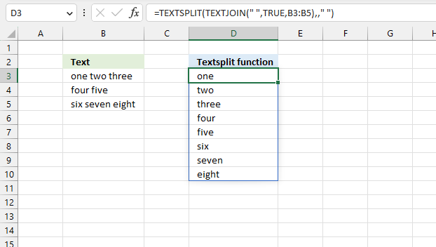
Join the cells using the TEXTJOIN function before splitting the strings.
Formula in cell D3:
This workaround is fine if the total character length is not above 32767 characters.
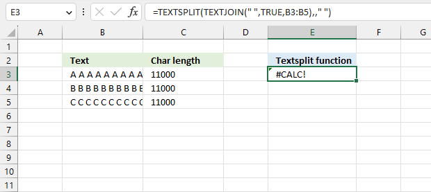
The image above shows a scenario where the total character count exceeds 32767 characters, the formula returns #CALC! error.
There is a workaround for this as well, the Excel 365 formula below doesn't have this limitation.
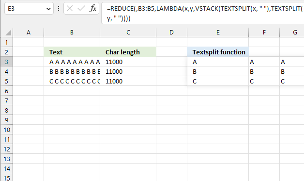
Excel 365 formula in cell E3:
Explaining the formula in cell E3
Step 1 - Split value into substrings
The TEXTSPLIT function splits a string into an array based on delimiting values.
Function syntax: TEXTSPLIT(Input_Text, col_delimiter, [row_delimiter], [Ignore_Empty])
TEXTSPLIT(y, " ")
Step 2 - Add arrays vertically
The VSTACK function combines cell ranges or arrays. Joins data to the first blank cell at the bottom of a cell range or array (vertical stacking)
Function syntax: VSTACK(array1,[array2],...)
VSTACK(TEXTSPLIT(x, " "),TEXTSPLIT(y, " "))
Step 3 - Create a LAMBDA function
The LAMBDA function build custom functions without VBA, macros or javascript.
Function syntax: LAMBDA([parameter1, parameter2, …,] calculation)
LAMBDA(x,y,VSTACK(TEXTSPLIT(x, " "),TEXTSPLIT(y, " ")))
Step 4 - Pass each cell value in cell range B3:B5 to the LAMBDA function
The REDUCE function applies each value in a cell range or array to a LAMBDA function, the result is a total value.
In this example, it is the opposite, each cell value is split into multiple substrings and the VSTACK function adds the arrays. The result is a larger array than the original size.
REDUCE(,B3:B5,LAMBDA(x,y,VSTACK(TEXTSPLIT(x, " "),TEXTSPLIT(y, " "))))
returns
{"A","A","A", ... ,"A";
"B","B","B", ... ,"B";
"C","C","C", ... ,"C"}
Useful links
TEXTSPLIT function - Microsoft
TEXTSPLIT function in Excel: split cells / text strings by delimiter
10. Concatenate cell values in a row into a single cell
This video demonstrates how to easily concatenate values in a single-row cell range into one cell. You will be surprised how easy it is to join cell values.
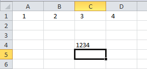
Here are the instructions for those of you that don't want to watch the video. The following picture shows you 4 values in row 1.
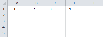 I know, it is a small number of values but the idea here is to show you the technique.
It is easier to demonstrate with a small number of values for obvious reasons.
Here is how to concatenate these values:
- Double press with left mouse button on cell C4
- Select cell range A1:D1
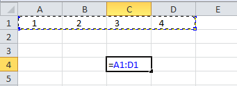
- Press function key F9 to convert the cell reference to values
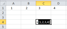
- Delete curly brackets: { and }
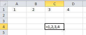
- Type CONCATENATE( and an ending parenthesis )
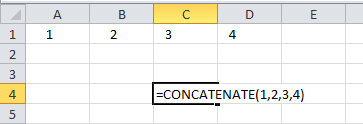
- Press Enter
Recommended reading:
Recommended articles
Add cell values to a single cell with a condition, no VBA in this article.
11. Concatenate cell values in a column into a single cell
This video explains the steps to join cell values in a column into a single cell. It also demonstrates how to use a delimiting character:
Here are the instructions for those of you that don't want to watch the video.
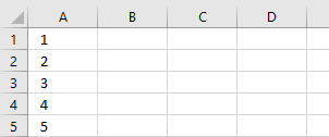 The picture to the right shows you a part of a larger range, A1:A50 containing numbers.
You can't see all the numbers in the picture for obvious reasons.
Let us concatenate these numbers in cell range A1:A50:
- Double press with left mouse button on cell C2.
- Type =TRANSPOSE(A1:A50)
- Press function key F9 to convert cell range to values.
- Delete curly brackets and equal sign.
- Type =CONCATENATE( in front of all characters in the formula bar.
- Type an ending parentheses ) at the very end
=CONCATENATE(1, 2, ... , 50) - Press Enter.
Here is an image of all concatenated numbers:
The TRANSPOSE function changes the cell reference from a vertical cell range to a horizontal cell range.
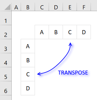 A vertical cell range has a semicolon as a delimiting character and that won't work with the CONCATENATE function.
A horizontal cell range has a comma as a delimiting character, the CONCATENATE function lets you enter arguments with a comma delimiter so this works fine.
It really depends on your regional settings, some countries use the semicolon as a delimiting character between arguments in an Excel function.
Recommended article:
Recommended articles
This article demonstrates how to find a value in a column and concatenate corresponding values on the same row. The […]
12. Concatenate a multi-column and multi-row cell range
This video shows you how to join values in a multi-column and multi-row cell range into one cell:
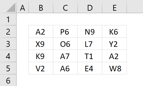
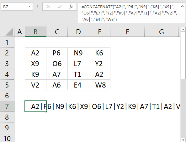
The following picture shows you values in cell range B2:E5.
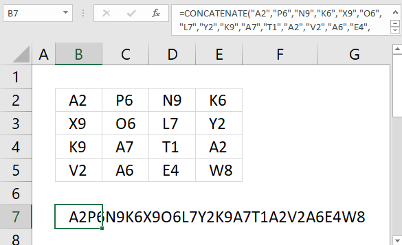
- Double press with left mouse button on cell B7.
- Type an equal sign = and then select cell range B2:E5 with your mouse.
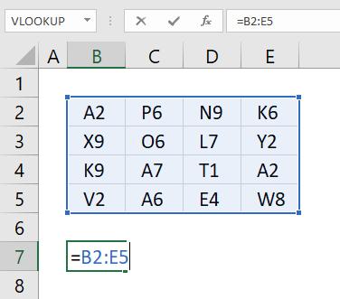
- Press F9 to convert cell reference to values.
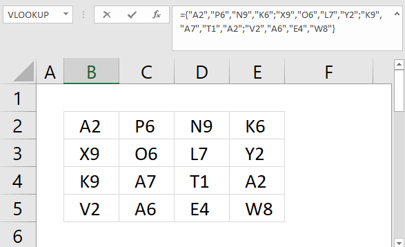
- Delete the equal sign and the curly brackets {}, then press Enter.
- Select cell B8
- Press CTRL + H to search and replace values, search for ; and replace with ,
- Press with left mouse button on "Replace" button.
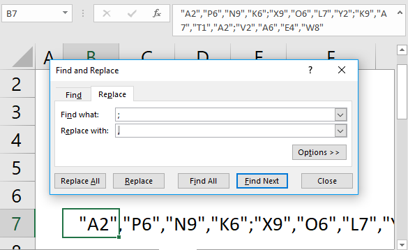
- Type CONCATENATE( in front of all characters in cell F2 and en ending parentheses after all characters
- Press Enter
Recommended post:
Recommended articles
This article demonstrates Excel formulas that extract unique distinct values from a cell range and concatenates the values using any […]
13. Create delimiting character
It would be great if we could have a special character separating our values.
Here is how:
- Double press with left mouse button on cell B8.
- Type =B2:E5&"|"
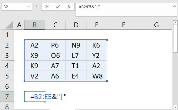
- Press function key F9 to convert cell reference to values.
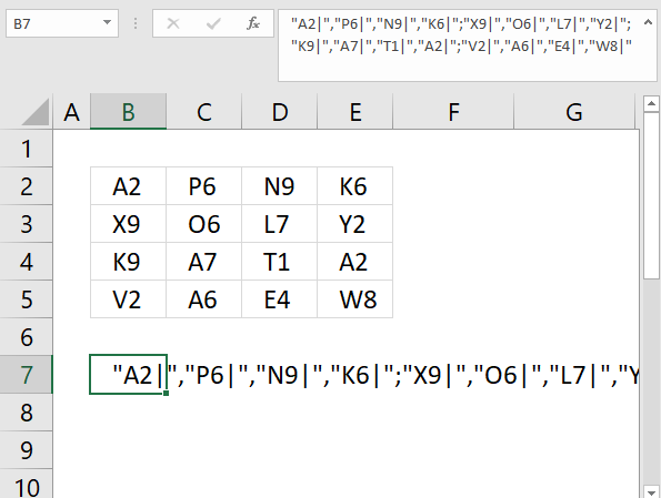
- Delete the equal sign and then press Enter.
- Select cell B8 again.
- Press CTRL + H to "Search and Replace".
- Search for a semicolon and replace with a comma, press with left mouse button on "Replace" button.
Do not press with left mouse button on "Replace All", this will replace values in all cells in your workbook.
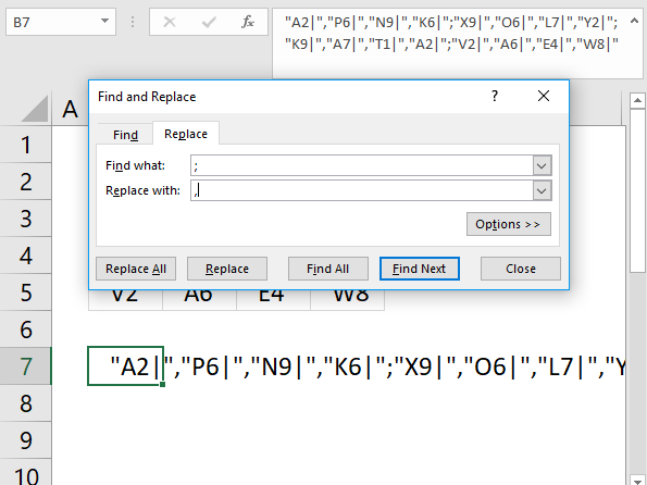
- Delete curly brackets and the last delimiting character.
- Type CONCATENATE( in front of all characters in cell B8 and en ending parentheses after all characters.
- Press Enter.
14. Concatenate unique distinct values - Excel 2019 formula
The new TEXTJOIN function in Excel 2019 lets you do some amazing things with arrays. This post demonstrates how to extract unique distinct values from a single column and concatenate the result into one cell.
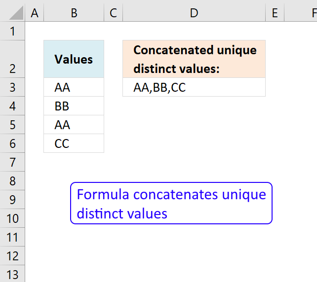
The following picture shows you 4 values in column B. Value "AA" has a duplicate in cell B5. Unique distinct values are all values except duplicates.
Array formula in cell D3:
Tip! You can use the UDF I made if you don't have Excel 2019 and can't use the TEXTJOIN function.
Recommended article
Recommended articles
Joining multiple cell values in Excel is not easy, for example, the CONCATENATE function allows you to only reference a […]
1.1 How to enter an array formula
- Double press with left mouse button on cell D3
- Copy/Paste above formula to cell D3
- Press and hold CTRL + SHIFT
- Press Enter once
- Release all keys
Your formula has now a beginning and ending curly bracket, like this:
Don't enter these characters yourself, they appear automatically if you followed the above steps.
Recommended article
Recommended articles
Array formulas allows you to do advanced calculations not possible with regular formulas.
1.2 Explaining array formula in cell D3
Step 1 - Match values with themselves
MATCH(B3:B6, B3:B6, 0)
becomes
MATCH({"AA"; "BB"; "AA"; "CC"}, {"AA"; "BB"; "AA"; "CC"},0)
and returns {1;2;1;4}
The MATCH function returns the relative position of a value in an array. It only returns the position of the first found value.
Value "AA" is found on the first position, so the first value in the array is 1. {1;2;1;4}
Value "BB" is found on the second position, so the second value in the array is 2. {1;2;1;4}
Value "AA" is found on the first position, so the third value in the array is 1. {1;2;1;4}
Value "CC" is found on the fourth position, so the fourth value in the array is 4. {1;2;1;4}
Recommended article
Recommended articles
Identify the position of a value in an array.
Step 2 - Compare array with relative positions
MATCH(B3:B6, B3:B6, 0)=MATCH(ROW(B3:B6), ROW(B3:B6))
returns {TRUE;TRUE;FALSE;TRUE}
This array tells us if a value is a duplicate or not. FALSE indicates a duplicate and we don't want that in the final result.
Step 3 - Filter unique distinct value
IF(MATCH(B3:B6, B3:B6, 0)=MATCH(ROW(B3:B6), ROW(B3:B6)), B3:B6, "")
returns {"AA";"BB";"";"CC"}
Recommended article
Recommended articles
Checks if a logical expression is met. Returns a specific value if TRUE and another specific value if FALSE.
Step 4 - Concatenate values
TEXTJOIN(", ", TRUE, IF(MATCH(B3:B6, B3:B6, 0)=MATCH(ROW(B3:B6), ROW(B3:B6)), B3:B6, ""))
returns AA,BB,CC.
The first argument in the TEXTJOIN function lets you specify the delimiting character. The second argument if you want to ignore empty strings. The third argument is the values you want to concatenate.
Recommended article
Recommended articles
What is the TEXTJOIN function? The TEXTJOIN function allows you to combine text strings from multiple cell ranges and also […]
15. Concatenate unique distinct values (VBA)
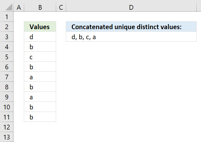
The formula in cell D3 contains a User Defined Function that extracts unique distinct values concatenated, you have the option to specify the delimiting character in the second argument.
The formula is a regular formula, however, you need to copy the code below and paste it to a code module in your workbook before you use it.
2.1 VBA code
'Name User Defined Function (UDF) and specify parameters
Function UniqConcat(rng As Range, str As String)

'Dimension variables and declare data types
Dim ucoll As New Collection, Value As Variant, temp As String

'Enable error handling, this is necessary because an error is returned when a duplicate string is added to the collection variable
On Error Resume Next

'Iterate through all values in range object rng
For Each Value In rng

    'Check if number of characters in variable Value is more than 0 (zero), if so convert value to string and then add converted value to collection variable
    If Len(Value) > 0 Then ucoll.Add Value, CStr(Value)

'Continue with next value
Next Value

'Disable error handling
On Error GoTo 0

'Iterate through values in collection variable ucoll
For Each Value In ucoll

    'Append value to variable temp and delimiting character
    temp = temp & Value & str

'Continue with next value
Next Value

'Remove last character from variable temp which is a delimiting character.
temp = Mid(temp, 1, Len(temp) - Len(str))

'Return string to cell in worksheet
UniqConcat = temp

End Function
2.2 Where to put the code?
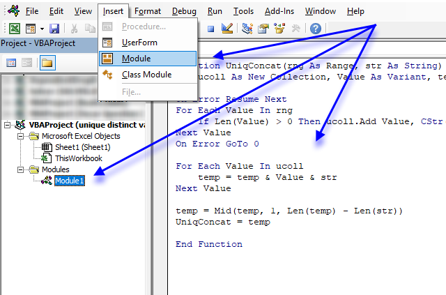
- Press Alt + F11 to open the VB Editor.
- Press with mouse on "Insert" on the menu.
- Press with mouse on "Module".
- Copy above code.
- Paste to code module.
- Exit VB Editor and return to Excel.
16. Concatenate unique distinct values - Excel 365
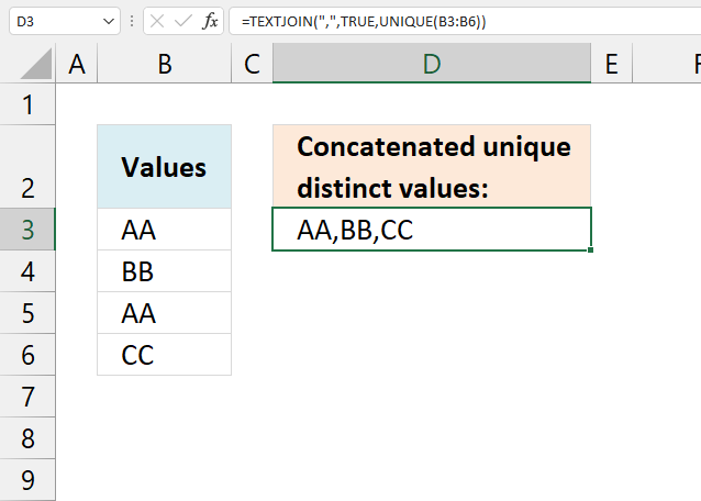
Formula in cell D3:
=TEXTJOIN(",", TRUE, UNIQUE(B3:B6))
4.1 Explaining formula in cell D3
Step 1 - Extract unique distinct values
The UNIQUE function returns unique distinct values and is a new function for Excel 365 users.
UNIQUE(B3:B6) returns {"AA";"BB";"CC"}
Step 2 - Concatenate unique distinct values
The TEXTJOIN function allows you to combine text strings from multiple cell ranges and also use delimiting characters if you want.
TEXTJOIN(delimiter, ignore_empty, text1, [text2], ...)
TEXTJOIN(",", TRUE, UNIQUE(B3:B6)) returns "AA,BB,CC" in cell D3.
17. Concatenate unique distinct values - Earlier Excel versions
Formula in cell D3:
=LOOKUP(2,1/(COUNTIF($D$2:D2,$B$3:$B$6)=0),$B$3:$B$6)
This formula is explained here. Copy cell D3 and paste to cells below as far as needed.
4.1 Concatenate values manually
Step 1 - Create a cell reference to unique distinct values
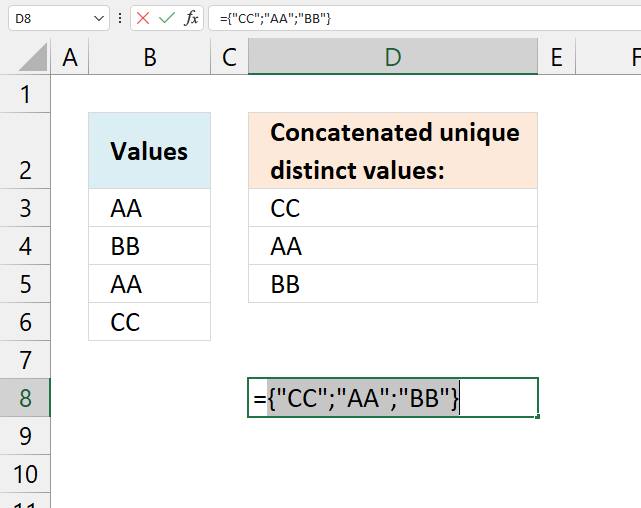
Double press with left mouse button on cell D8. Press = (equal sign) and select with mouse cell range D3:D5. Alternatively, type D3:D5.
=D3:D5
Don't press Enter yet.
Step 2 - Convert values in cell range to array values
Press F9 on your keyboard to convert cell reference D3:D5 to actual values.
={"CC";"AA";"BB"}
Step 3 - Remove curly brackets and equal sign
={"CC";"AA";"BB"} becomes "CC";"AA";"BB"
Press Enter.
Step 4 - Find and Replace
Select cell D8.
Press CTRL + H to open the "Find and Replace" dialog box.
Press with the left mouse button on tab "Replace" located on the dialog box.
Type ";" in "Find what:" field, see image below.
Type , in "Replace with:" field, see the image below.
Press with left mouse button on "Replace" button.
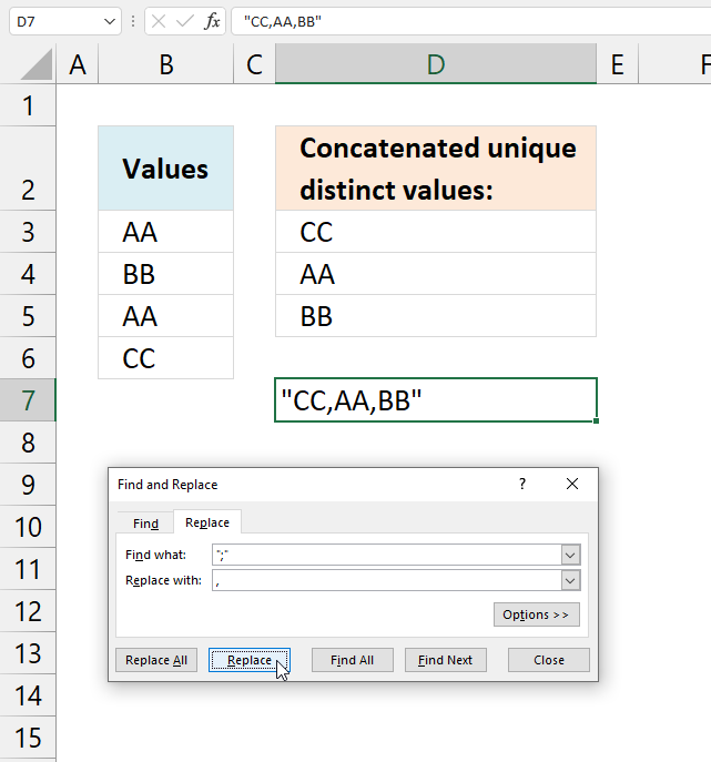
Press with left mouse button on "Close" button.
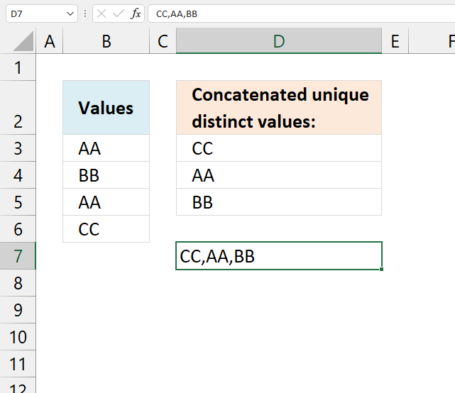
Step 4 - Remove double quotes
18. Function not working
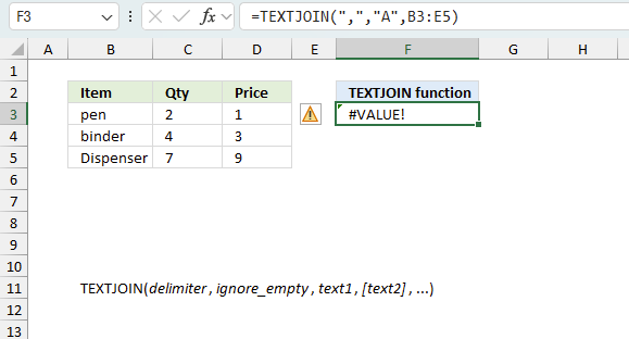
The TEXTJOIN function returns
- #VALUE! error if you use a non-boolean value in the second argument ignore.
- #NAME? error if you misspell the function name.
- propagates errors, meaning that if the input contains an error (e.g., #VALUE!, #REF!), the function will return the same error.
18.1 Troubleshooting the error value
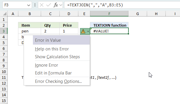
When you encounter an error value in a cell a warning symbol appears, displayed in the image above. Press with mouse on it to see a pop-up menu that lets you get more information about the error.
- The first line describes the error if you press with left mouse button on it.
- The second line opens a pane that explains the error in greater detail.
- The third line takes you to the "Evaluate Formula" tool, a dialog box appears allowing you to examine the formula in greater detail.
- This line lets you ignore the error value meaning the warning icon disappears, however, the error is still in the cell.
- The fifth line lets you edit the formula in the Formula bar.
- The sixth line opens the Excel settings so you can adjust the Error Checking Options.
Here are a few of the most common Excel errors you may encounter.
#NULL error - This error occurs most often if you by mistake use a space character in a formula where it shouldn't be. Excel interprets a space character as an intersection operator. If the ranges don't intersect an #NULL error is returned. The #NULL! error occurs when a formula attempts to calculate the intersection of two ranges that do not actually intersect. This can happen when the wrong range operator is used in the formula, or when the intersection operator (represented by a space character) is used between two ranges that do not overlap. To fix this error double check that the ranges referenced in the formula that use the intersection operator actually have cells in common.
#SPILL error - The #SPILL! error occurs only in version Excel 365 and is caused by a dynamic array being to large, meaning there are cells below and/or to the right that are not empty. This prevents the dynamic array formula expanding into new empty cells.
#DIV/0 error - This error happens if you try to divide a number by 0 (zero) or a value that equates to zero which is not possible mathematically.
#VALUE error - The #VALUE error occurs when a formula has a value that is of the wrong data type. Such as text where a number is expected or when dates are evaluated as text.
#REF error - The #REF error happens when a cell reference is invalid. This can happen if a cell is deleted that is referenced by a formula.
#NAME error - The #NAME error happens if you misspelled a function or a named range.
#NUM error - The #NUM error shows up when you try to use invalid numeric values in formulas, like square root of a negative number.
#N/A error - The #N/A error happens when a value is not available for a formula or found in a given cell range, for example in the VLOOKUP or MATCH functions.
#GETTING_DATA error - The #GETTING_DATA error shows while external sources are loading, this can indicate a delay in fetching the data or that the external source is unavailable right now.
18.2 The formula returns an unexpected value
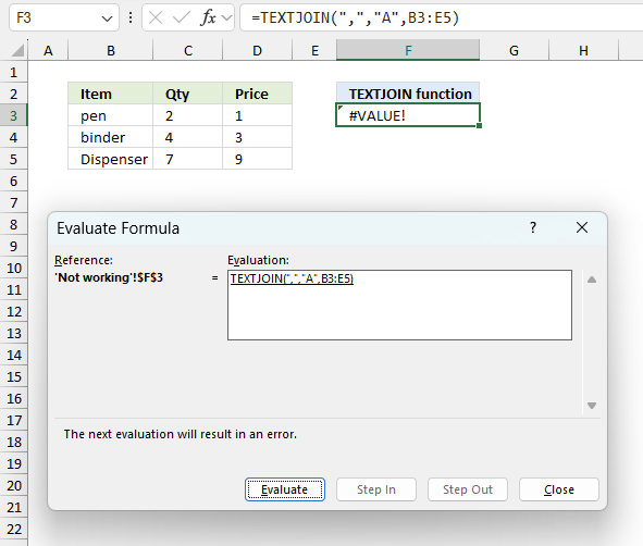
To understand why a formula returns an unexpected value we need to examine the calculations steps in detail. Luckily, Excel has a tool that is really handy in these situations. Here is how to troubleshoot a formula:
- Select the cell containing the formula you want to examine in detail.
- Go to tab “Formulas” on the ribbon.
- Press with left mouse button on "Evaluate Formula" button. A dialog box appears.
The formula appears in a white field inside the dialog box. Underlined expressions are calculations being processed in the next step. The italicized expression is the most recent result. The buttons at the bottom of the dialog box allows you to evaluate the formula in smaller calculations which you control. - Press with left mouse button on the "Evaluate" button located at the bottom of the dialog box to process the underlined expression.
- Repeat pressing the "Evaluate" button until you have seen all calculations step by step. This allows you to examine the formula in greater detail and hopefully find the culprit.
- Press "Close" button to dismiss the dialog box.
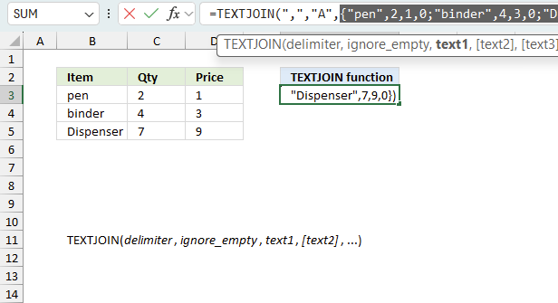
There is also another way to debug formulas using the function key F9. F9 is especially useful if you have a feeling that a specific part of the formula is the issue, this makes it faster than the "Evaluate Formula" tool since you don't need to go through all calculations to find the issue.
- Enter Edit mode: Double-press with left mouse button on the cell or press F2 to enter Edit mode for the formula.
- Select part of the formula: Highlight the specific part of the formula you want to evaluate. You can select and evaluate any part of the formula that could work as a standalone formula.
- Press F9: This will calculate and display the result of just that selected portion.
- Evaluate step-by-step: You can select and evaluate different parts of the formula to see intermediate results.
- Check for errors: This allows you to pinpoint which part of a complex formula may be causing an error.
The image above shows cell reference B3:D5 converted to hard-coded value using the F9 key.
Tips!
- View actual values: Selecting a cell reference and pressing F9 will show the actual values in those cells.
- Exit safely: Press Esc to exit Edit mode without changing the formula. Don't press Enter, as that would replace the formula part with the calculated value.
- Full recalculation: Pressing F9 outside of Edit mode will recalculate all formulas in the workbook.
Remember to be careful not to accidentally overwrite parts of your formula when using F9. Always exit with Esc rather than Enter to preserve the original formula. However, if you make a mistake overwriting the formula it is not the end of the world. You can “undo” the action by pressing keyboard shortcut keys CTRL + z or pressing the “Undo” button
18.3 Other errors
Floating-point arithmetic may give inaccurate results in Excel - Article
Floating-point errors are usually very small, often beyond the 15th decimal place, and in most cases don't affect calculations significantly.
'TEXTJOIN' function examples
This post explains how to lookup a value and return multiple values. No array formula required.
This blog article describes how to split strings in a cell with space as a delimiting character, like Text to […]
In this blog post I will demonstrate methods on how to find, select, and deleting blank cells and errors. Why […]
Functions in 'Text' category
The TEXTJOIN function function is one of 29 functions in the 'Text' category.
Excel function categories
Excel categories
116 Responses to “How to use the TEXTJOIN function”
Leave a Reply
How to comment
How to add a formula to your comment
<code>Insert your formula here.</code>
Convert less than and larger than signs
Use html character entities instead of less than and larger than signs.
< becomes < and > becomes >
How to add VBA code to your comment
[vb 1="vbnet" language=","]
Put your VBA code here.
[/vb]
How to add a picture to your comment:
Upload picture to postimage.org or imgur
Paste image link to your comment.



Wont work.
A1:A50 will return a row array.
You will need to type =transpose(a1:a50) in cell b1 , say f9, delete the curly brackets and type concatenate
Hi, this does not work in my excel. When I type =TRANSPOSE(A1:A7) in the formula, it brings only the first cell value. On press of F9 also, no change in the value. I tried the steps mentioned by you, but could not make it. Please help me on this. Thanks in advance..
Nandhini,
Type TRANSPOSE(A1:A7) in a cell. Do not press Enter. Press F9.
Oscar, thanks a lot. It works. With a demo you replied and helped me to get knowledge on it. I really appreciate your assistance and thank you so much for your help.
=Transpose() is unnecessary. Just type =A1:A7 and hit F9 BEFORE hitting enter, to get the corresponding values in an array'd list.
Sam,
Thanks for commenting!
It works with my regional settings in excel 2007.
Oscar, In the English version the row array has a ; as a separator and a column array has a , as a separator.
=A1:A10 give ={"name1";"name2";.....;"name10"} etc
Great tip, Oscar. Surprised that Microsoft didn't fix this in the Excel 2010, but go figure. Sam, I think I had the same problem as you and I was running the evaluate (F9) by selecting just the range and not the full TRANSPOSE(A1:A50) in the formula. If you run the evaluate on just the evaluated range of A1:A50, it will keep the semi-colon separator and not use the comma. But if you run the F9 by selecting the function and the range [TRANSPOSE(A1:A50)], it should work. Awesome tip, I have run into this issue many times before. Glad I now know the fix.
Michael,
Thanks!!
HI Oscar, THANKS for the tip on "Create delimiting character"! One quick question, how do I remove the space between the comma after A1 and B1? So it looks like A1,B1,C1....
Thanks!
FuWaye
FuWaye,
=TRANSPOSE(A1:A50)&","
Great tip thanks! On Office for Mac, use command+'=' instead of F9
Thanks very much. Especially the extra bit adding a separator. Will save me a lot of time.
I had to play with it a bit in Office 2010, but that F9 trick saved me hours.... Nice job !!!
Damien, Ross and Mark
Thanks!!
Thanks man! Great tip!
Nice.Thanks for your help. Only annoying thing is that the formula is limited on 8592 caracters or something like this. otherwise is just perfect with F9 function. Good job. 10x
There's another way to do it. It's a bit more cumbersome but it updates automatically (which this won't do for me) and you don't need to go through the process of selecting each cell (which can take quite awhile if there are a lot of them).
In a new cell, alongside the ones you will concatenate or anywhere else that there's enough space, set it equal to the first cell. Then in the next cell, concatenate that new cell and the second cell. Now just drag it all the way to the end and they'll all be concatenated. (I did it the other way around from the end to the beginning so the resulting string was at the beginning but it should work either way.
Like I said, it's a bit cumbersome but it updates and you don't have to select all the cells. As a plus, you can add onto it or take away from it simply by dragging without having to edit the formula again.
To concatenate e.g. A2 to A100,
the OFFSET function allows for an easier and more robust solution:
In cell B2, write:
=OFFSET(B2, -1, 0) & OFFSET(B2, 0, -1)
This will concatenate the content in the above cell, B1, and the left hand cell, A2.
Using the small cell handle in B2's bottom right hand corner, drag downwards to copy the cell as many rows as desired. In B100, the content of A2, A3, A4 ... A100 will be concatenated.
In comparison to Richard's method, this is more robust because each cell only references itself. Thus, removing a row or reordering/sorting rows will not yield a #REF! error.
In the above example, note that the cell B1 should be left empty.
This was very helpful. Thank you for sharing!
Thanks Richard. It's really nice trick.
@Richard,
If you do the repeatd concatenations downward, you can display the last one using this formula (adjust the specified ranges as needed)...
=LOOKUP(2,1/(B1:B65535""),B:B)
no need of OFFSET and similars. just use the following:
1- make B1 blank
2- on B2 enter: "= B1&A1" (obviously without the " ")
3- Press with left mouse button on B2, get the cell handle and drag all the way to B51
The concatenated string is in B51
Cheers... Jorge
Richard,
I believe this post describes the same method:
https://www.get-digital-help.com/concatenate-cell-values-in-excel/
You can also use an user defined function to concatenate values:
https://www.contextures.com/rickrothsteinexcelvbatext.html
[...] פתרון המשתמש בכלים הקיימים באקסל – קראתי אותו בעמוד הבא. החסרון של פיתרון זה הוא חוסר אפשרות [...]
Great tip! If only I had known this years ago.
You are a genius.
worked great
lets take over the world
Brilliant!
Awesome, you just saved me hours of work!!!!
thanks..gr8 workaround.
This post was sickeningly awesome.
Awesome seriously ... frustration is abated. My work needed I concatenate range of cells with comma. Works amazing. My regional settings needs the =transpose(a1:150)&","
Thanks much
Hello,
thanks a lot for these steps.
It helps do many things faster as other users wrote.
Michal Kalián,
Thanks for commenting!
Genius! excellent
So happy to have found this :)
Sam and Caz,
I am happy you like it!
My problem was a continuously expanding dataset of term deposits from which some values needed to be extracted to a single text string based on date for inclusion in a report. Let's say the dataset occupied columns A, B, C and D. In column E, I created an IF() function to return the report output, including a delimiter, for that entry if it lay in the wanted date range and a null "" string if it did not. The problem then was to concatenate the results in column E. I solved this by concatenating the result in each row with the value in the subsequent row thus, in cell E1, the formula looks like =CONCATENATE(IF(....),E2) where IF(....) is the formula for the output based on row 1. I then used fill down to replicate this formula in cells (E2:En) and the output in cell E1 then contains all that I need for my report. Works for any number of rows but will become slow if too many rows produce wanted output.
Alan,
Thanks for sharing!
[...] Publisher More from patrick dhungel: Python Miscellaneous kindle Sort Share https://www.get-digital-help.com 3 minutes [...]
What if you had multiples columns which you wanted to concatenate individually?
A1 A2
B1 B2
C1 C2
.. ..
A1, B1, C1 etc
A2, B2, C2 etc
Manually doing F2 F9 across multiple columns would be painful. Is there formula or macro that can automate this?
The point of this page is to do it without a macro (vba) and, short of writing one, I don't think it can be done for multiple columns. As to the pain, the method that I and others have used involves putting a formula in only one cell, the top cell of the leftmost column, then using fill down to replicate it in the other cells of that column. Once that is done, select the column that now contains the formulas and fill right to replicate the whole column for the remaining columns. Unless your spreadsheet is huge, this should be relatively quick and easy. If your columns are not adjacent, you will have to use copy and paste instead of fill right.
Cube,
Rick Rothstein (MVP - Excel) posted a user defined function here:
https://www.get-digital-help.com/concatenate-cell-values-in-excel/#comment-5003
Great tip, its what Im looking for
I've tried to apply for multiple row but not success. could you kindly guide how to do if it is possible
data as follow:
A B C result
1 100 200 300 100200300
2 400 500 600 400500600
3 700 800 900 700800900
........................
I have a lots of rows, there is any way to apply for multiple rows?
I means, we dont need go to each cell then press F9 then delete curly brackets.
tks so much
DTNAM,
I recommend using Rick Rothstein's (MVP - Excel) user defined function here:
https://www.get-digital-help.com/concatenate-cell-values-in-excel/#comment-5003
tks so much, I just want to find out any tips to solve it
You should add a nice formula to have cells report their own reference as a string eg:
=CONCATENATE(SUBSTITUTE(ADDRESS(1,COLUMN(),4),"1",""),ROW())
Then you can easily create a string of references for further concatenation eg: put my first formula in A1 and copy the following formula into cell B1 and then copy that through to J1. The desired string is then in J1
=CONCATENATE(A1,",",CONCATENATE(SUBSTITUTE(ADDRESS(1,COLUMN(),4),"1",""),ROW()))
Two formula, no typing: copy paste x3 Done.
richard,
Thank you for you contribution.
I made a similar post a while ago that concatenates values:
https://www.get-digital-help.com/concatenate-cell-values-in-excel/
@Rick Rothstein (MVP - Excel)
I found some confuse your recommend as below;
"@Richard,
If you do the repeatd concatenations downward, you can display the last one using this formula (adjust the specified ranges as needed)...
=LOOKUP(2,1/(B1:B65535""),B:B)"
I would like to repeated concatenations downward, as example problem
A B C D expected result
1 2 3 4 1234
M O D C MODC
I follow your recomment
Step 1 = A1:D1 and press F9
Step 2 = {1,2,3,4}
Step 3 = I type concatenate in formula field
By the way, however, I will repeated this formula in new cell (B2:D2) to get above expected result
thank you
Of course we wouldn't need any such tricks if MS wrote a DECENT concatenate function where you simply passed in a range and an optional delimiter.
I believe that the MCONCAT function (3rd-party add-on) does just that. (Or I'd write my own UDF in most cases)
But if you are still wanting to create CONCATENATE formulas without VBA then certainly the little F9 trick can save time. Thanks !
[…] פתרון המשתמש בכלים הקיימים באקסל – קראתי אותו בעמוד הבא. החסרון של פיתרון זה הוא חוסר אפשרות […]
RE: Concatenate a cell range without vba in excel
Thank you! WORKS WONDERFULLY. I'm not programming-literate so, although I have had occasion to try to understand & tackle VBA solutions, a good Macro saves me tons of time & aggravation.
(Note: The only problem I have is that I have numerous cells in the range that very frequently have null (0) values, but I DON'T want to see any of the zeros in the concatenated string/result (& there's no need for anything in the string to indicate the place that 0 would occupy). (I've set my worksheet Display Options to NOT show 0 values.) Any suggestions would be welcome & appreciated; but as it is, I can easily work around this minor issue. SO THANK YOU FOR A GREAT TIP My work-around for the 0's is to just add a step between your step 6. & 7.(below), to remove any "0" values from the transposed formula, which is easy because in my particular data they necessarily occur at the end of the string.)
BELOW is the portion of your post that helped me out so effectively, & the TRANSPOSE part under step 2 was key for me :
... RE: Let´s concatenate these values:
1.Select cell B1.
2.Type =A1:A50 in formula bar.
Edit: Depending on your regional settings, try this: =TRANSPOSE(A1:A50)
3.Press F9.
4.Delete curly brackets in formula bar.
5.Type =Concatenate( in front of all characters in formula bar.
6.Type ) at the end in formula bar.
7.Press Enter
Formula in cell B1:
=CONCATENATE("A1","B1","C1","D1","E1","F1", ...) + ENTER
Connie,
Thank you!
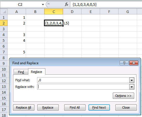
Use Find and Replace to remove null values (CTRL + H)
Thank you so much for this.
It has helped me with a project I am working.
Such a timesaver.
It has opened my mind to so many ideas, as well.
Thanks. Well done!!!
Gregg
Gregg Harris,
Thanks for commenting!
Hi--I am not getting "" around my numbers...they are just commas...is there something Im missing?
sharon,
No, you are right. Only text values have quotation marks. But you can concatenate numbers also.
Hi,
I really liked this solution.
Was wondering how to deal with a dynamic range (e.g the initial formula was =transpose(A1:A50)..., but it may become A1:60 and I still want all values concatenated with the "," delimiter.
Thanks
Sam,
Yes you can.
Get the Excel *.xlsx file
Concatenate-a-dynamic-named-range-and-a-table.xlsx
In Column A, rows 1 to 5, type the following:
red
yellow
blue
green
orage
In cell B2:
=IF(ROW()=2,A1&OFFSET(B2,-1,0)&","&OFFSET(B2,0,-1),OFFSET(B2,-1,0)&","&OFFSET(B2,0,-1))
Drag this formula down to cell B5.
Cell B5 will now contain the string "red,yellow,blue,green,orage"
Nuovella,
Yes, I have made something similar:
https://www.get-digital-help.com/concatenate-cell-values-in-excel/
Thanks Oscar.
Hi OSCAR:
Luckly found this site and wonderful.
I have a work sheet called: Data. Column A has dates and column B has related data. New data is being added weekly based at top (current at top and older downward). Then I create chart that shows me line chart of all data (last 10 years or so), up to here no problem and I am good.
Problem I have when need to create chart of latest one year data or latest 2 years data. In this case I need to change chart series reference cell. My start date always starts at A7. What I am trying to do is enter number of weeks (assuming 52 w/yr multiply by number of years) in one cell then CONCATENATE A and number of weeks to get end date. Then concatenate Start date A7 and End date (concatenated after entering number of weeks) to get a Date range e.g. A7:A59. Up to here I am doing ok (may be I am wrong). How to link this concatenated range to chart data series, so chart will show me graph of required date range.
Any help would be appreciated. Spent almost one week searching on web to find any related help but no successful.
Here is data of my table:
Date=Colum: A Data=Column B
=================================
11/03/2014 684249
04/03/2014 656664
25/02/2014 637838
18/02/2014 657075
11/02/2014 617237
04/02/2014 602247
28/01/2014 608056
21/01/2014 663764
14/01/2014 664721
07/01/2014 630115
Kam,
I have a work sheet called: Data. Column A has dates and column B has related data. New data is being added weekly based at top (current at top and older downward). Then I create chart that shows me line chart of all data (last 10 years or so), up to here no problem and I am good.
Problem I have when need to create chart of latest one year data or latest 2 years data. In this case I need to change chart series reference cell. My start date always starts at A7.
I understand you up to this point. Anyway, perhaps this post is helpful: Make a dynamic chart for the most recent 12 months data
Oscar, thanks a lot for help. Found out way through your help.
Good work, keep it up.
Regards
Kam
Kam,
thank you.
Dear Oscar
I have the following entries in two adjacent columns:
ColA,ColB
a,one
a,two
b,three
b,four
c,five
c,six
I need concatenation of colB entries in colC, as follows:
C1:one,two
C3:three,four
C5:five,six
Thanks
I need array formula solution and not VBA code or UDFs.
Thanks
SridharVenu,
This is a regular formula.
I thought you could use a spare sheet to construct a concatenate command.
I wanted to join all the cells from D2 to EM2.
But how to get the x2,y2,z2,aa1,ab1, etc.
You can convert numeric references to cell IDs using "address"
for me I needed D2 which is 2,4
I had a column A which I autofilled with 4,5,..143
To get the relative address, D2 without any $s, use 4 for the address type.
type this in B2 =address(2,A1,4)
Autofill down by double pressing in the little square at the bottom right of the cell.
Now build the list.
in d1 type =B1
in d2 type =D1 & "," & B2
Drag the autofill to the bottom and you will end up with all the cell names seperated by commas in D139
in c139 type ="=concatenate("&D139&")"
This is a bit weird because we are constructing an excel formula with strings that look like excel formula! :-)
The value of C139 will now be our big concatenation command.
Copy the cell and go to C2 on the sheet where you want the concatenate.
You now have to trick excel!
Paste value into the cell.
Excel thinks "This is a value so I'l better treat it as a literal string"
the value of C2 is now "=concatenate(B2,C3...."
Copy the cell and paste it back into C2.
Hurrah! The value of C2 is now the concatenation of all the cells that you wanted.
Autofill down to do the same to all the rows.
(This only saves typing if you have more than 30 or so columns to concatenate. :-)
Hope this is of use!
Alan Gunn
Awesome Trick!
It saved my time a lot...
Thanks!
I need t to merge rows in one of my excel sheets, so after long googling this simple function has been borned and I name it MergeCells(). Calling it is simple, select the range you want to merge, and set the delimiter.
Example:
MergeCells(A23:Q23, "-")
Public Function MergeCells(cellsRange As range, delimiter As String) As String Dim cell As range Dim mergedCells As String mergedCells = "" For Each cell In cellsRange mergedCells = mergedCells & delimiter & cell.Value Next cell MergeCells = Right(mergedCells, Len(mergedCells) - 1) End FunctionHi,
to concatenate a column (or row) range, like, say, the strings in A1 to A50 do this:
1- on B2 enter: "= B1&A1" (obviously without the " ")
2- Press with left mouse button on B2 and drag all the way to B51
The concatenated string is in B51
Cheers... Jorge
[email protected]
=TRANSPOSE etc doesnt give me the ; in the final cell.
How to concatenate whole row leaving the blank cells with a delimiter ","
How to concatenate whole row leaving the blank cells with a delimiter ","
with formula
Worked just great for me. Saved me a lot of re-typing. Thanks!!!!
All I had to do, was to follow the well documented instructions.
Hello to every one, since I am in fact keen of reading this blog's post to be updated regularly.
It consists of nice information.
Hello, I have one Job card file, one job card have different different items description; may be it will come 6 line or 10 line of item description like that, I need this item details should be in one cell based on the Job Card No. (Job card no will come 1 2 3 4 5 6 7............ Like that) Job card No + 10 Lines Items descriptions in one cell, then I can easily understand that job card have what are the items should be make. This file come more than 3000 job card also. that mean if I will put some equation with =CONCATENATE after I drag first the end, I can get the report like that or not in excel ?
This is Sinu Mathew, My Job Card File coming like this
Job Card No JC Dt- Delivery Due Dt Customer Name Bx Type Qty in Nos
67 13-04-16 17-06-16 Mathew DC-Bg-1x4-B 60
157 26-04-16 03-06-16 Govind ML-2x2x3 300
157 26-04-16 03-06-16 Govind Printing 1
162 24-04-16 29-05-16 Menon BK 1852
162 24-04-16 29-05-16 Menon WB-5x5x2-V 832
162 24-04-16 29-05-16 Menon OB-WB-5X5X2-P 832
162 24-04-16 29-05-16 Menon Printing 1
168 27-04-16 28-05-16 Midun Calender 6
168 27-04-16 28-05-16 Midun Acc-FG 4
168 27-04-16 28-05-16 Midun PYM-19 Pcs 4
168 27-04-16 28-05-16 Midun WB-3x3x3-V 3
168 27-04-16 28-05-16 Midun OB-WB-3x3x3-P 3
168 27-04-16 28-05-16 Midun ML-3x3x3 4
168 27-04-16 28-05-16 Midun SL-1x6 15
168 27-04-16 28-05-16 Midun DC-L Lantern-1X8-B 6
168 27-04-16 28-05-16 Midun B GE 6
168 27-04-16 28-05-16 Midun Ham-20x20x20 2
168 27-04-16 28-05-16 Midun DC-L Lantern-1X8-B 2
168 27-04-16 28-05-16 Midun DC-M Lantern-1x2-B 2
168 27-04-16 28-05-16 Midun DC-S Lantern-1X1-B 2
168 27-04-16 28-05-16 Midun SB-1x2 2
168 27-04-16 28-05-16 Midun BK 2
168 27-04-16 28-05-16 Midun Midhun 1
168 27-04-16 28-05-16 Midun SB-4x4x1 1
168 27-04-16 28-05-16 Midun DC-L Lantern-1X8-B 1
168 27-04-16 28-05-16 Midun BK-3x2 1
168 27-04-16 28-05-16 Midun SB-1x4 1
168 27-04-16 28-05-16 Midun S GE 1
168 27-04-16 28-05-16 Midun Ham-30x25 1
168 27-04-16 28-05-16 Midun Pym-19 Pcs 1
168 27-04-16 28-05-16 Midun DC-M Lantern-1x2-B 1
168 27-04-16 28-05-16 Midun DC-L Lantern-1X8-B 1
hi sir, a1:a50 contain test data, b1:b50 contain digit. i want to print a1:a50 text data into c1 cell giving range(0 to1000), c2 range 1001 to 2000 etc based on b1:b50
thanks!
helped me out for work today
Hi Oscar,
I have one cell with some string and need to concanetate it with 38 cells... how may I do it plz help!
AIAP38KE CON-SPSSC2P- CON-SPSSC4P- CON-SPSSC4S- CON-SPSSCS- CON-SPSSRTF- CON-SPSSS2P- CON-SPSSS4P- CON-SPSSSNE- CON-SPSSSNT- CON-SPSSSPB- CON-SSC2P- CON-SSC4P- CON-SSC4S- CON-SSCS- CON-SSCSS- CON-SSP4P- CON-SSP4S- CON-SSPC2- CON-SSPCS- CON-SSPNB- CON-SSPNE- CON-SSPNP- CON-SSPS2- CON-SSS2P- CON-SSSNE- CON-SSSNP- CON-SSSNT- CON-SSSW- CON-SSX4P- CON-SSX4S- CON-SSXC2- CON-SSXCS- CON-SSXNB- CON-SSXNE- CON-SSXNP- CON-SSXS2- CON-SSDR5- CON-SSDR7-
to elaborate...
I want the string "AIAP38KE"
with all the CON-XXx-"AIAP38KE"
[…] versions to excel 2016, however if you have excel 2016 you can now finally use the much easier TEXTJOIN function. Here is a larger range, A1:A50 with some […]
[…] This page helped with quickly making a long CONCATENATE list. […]
https://www.youtube.com/watch?v=QJ2O07EB80Q&feature=youtu.be
Great video!
I followed the instructions but when I type TEXTJOIN( in a cell I get an error "Ambiguous name detected: TEXTJOIN".
I am new to using Visual Basic so am probably doing something silly but it doesn't seem to recognize the TEXTJOIN function I've created
Any ideas?
josh,
This error occurs when there are multiple UDFs with the same name in a module.
Not working for me. Get VALUE! error
lesli
Can you post your formula here?
Also after finding the function, it commits to the SS all lowercase not upper. That is an alert to me as my other functions keep the exact name case format.
This is great. Is there a way to combine it with vlookup, please?
Gustavo,
Concatenate cell values based on a condition [No VBA]
I followed the instructions for TEXTJOIN unique values and got the curly brackets, but cell was empty.
It may have something to do with the fact that my array is a list of horizontal cells rather than vertical ?
I tried "column" instead of "row" in the the function but got "#value!"
Please help.
Can you post the formula?
Hello, nice, but can you try your formula with with 10000 records? It is working with 1000 but failing with 10000 as it is not removing the empty cells any more...
Tamas
Weird, you probably need a UDF.
If you are looking to remove the blanks, change the formula to the following:
=TEXTJOIN(", ", TRUE, IF(E8:E38="", "", IF(MATCH(E8:E38, E8:E38, 0)=MATCH(ROW(E8:E38), ROW(E8:E38)), E8:E38, "")))
I was doing this for range E8 to E38, should work for any range though with any number of blanks.
Hi - Thanks for posting this - as I've had to make my spreadsheet backwards compatible with older versions of Excel.
I've been using this UDF for some time but have found that myself and others receive an occasional error where the first line of code (Function TEXTJOIN1(delimiter As String, ignore_empty As Boolean, ParamArray cell_ar() As Variant)) is highlighted in the VB editor with the following error being thrown on Excel opening the file: "Automation error Catastrophic failure". I've done some research and have yet to figure out why this may be throwing an error on some machines intermittently and not others. Some posts point to using 'Range' instead of 'String' ... which I've tried with no luck.
Wasn't sure if anyone else had encountered this?
Thanks!
ASmyth
"Automation error Catastrophic failure"
That is an error I never have encountered or heard of before.
This StackOverflow page suggests a few solutions:
https://stackoverflow.com/questions/31888880/automation-error-catastrophic-failure-excel-vba
Your CONCATENATE and TRANSPOSE formulas are exactly what I needed! I've been getting SO annoyed trying to do this and your solution is perfect! You have totally made my day, thank you!
Thank you, Jenny.
Hi, I have used this formula {=TEXTJOIN(",",TRUE,IF(I2=$A$2:$A$4785,$B$2:$B$4785,""))} to link text from different cells which has worked for the most of my data, but for some I get the #Value error appear. I cannot see why I am getting this as the cells are formatted the same and there is nothing seemingly different. Any ideas?
Thanks and thanks for creating the above, its really useful
How can I Lookup and return unique distinct values concatenated into one cell. I prefer to have the VBA code as most users may not have latest office.
I also want it to update if a new data in eneterd in the source.
Is there a way to use the textjoin function with more than 3000 records?
Mike,
The TEXTJOIN function returns a #VALUE! error if the returned value has more than 32767 characters.
https://support.office.com/en-us/article/textjoin-function-357b449a-ec91-49d0-80c3-0e8fc845691c
There's a link for textjoin based on 1 criteria, and there's another link for textjoin with the condition that they're unique values, but how do I do both? For the sake of argument, my formula cell is J5. G5 has a customer ID. My formula is looking for a matching customer ID in range 'Reject Details'!$B$1:$B$500 to retrieve the corresponding part# in 'Reject Details'!$E$1:$E$500.
TEXTJOIN(", ",TRUE,IF($G5='Reject Details'!$B$1:$B$500,'Reject Details'!$E$1:$E$500,""))
The issue is that I'm trying to show what a customer buys, without getting "basket, basket, basket, basket, basket".
I have the same issue. Did you get any solution?
Hello,
I have used the VBA to add this formula to an older Excel. I have one issue with it though, blank columns return a #VALUE! error.
I use the formula to add all the items in rows in a range
=TEXTJOIN(" ",TRUEX5:X48)
Each column from X to BC has this formula in it. Not every column is used every day, but the product changes day by day. Is there a way to avoid this error if the column is blank?
I have found that if I make the delimiter "" then the error does not appear, but then I have spacing issues left behind.
Thanks for the VBA code. It solved my problem
Thank you for VBA code!!! Greetings from Lithuania! ;)
Asslam-O-Alikum!
In Excel 2016 I used the above given VB code for txetjoin function(TEXTJOIN(delimiter, ignore_empty, text1, [text2], ...), but for ignore_empty either True or False, it is not ignoring the empty cell the example is given below:
the formula used is
=textjoin(", ",TRUE,IF(I11:I15="✓",B11:B15," "))
& the result is
, , , M/S Sohail Engineering Corporation, Badami Bagh, Lahore.,
kindly guide me.
This is one of the best page I have seen with excellent step by step instructions in Layman language. Thank you so much.