How to use the LAMBDA function
What is the LAMBDA function?
The LAMBDA function lets you build custom functions using only regular Excel functions, no VBA is needed. These custom functions based on the LAMBDA function are available only in your workbook.
The Name Manager lets you create a unique easy to remember name for your custom LAMBDA function that allows you to reuse the complex formula across worksheets.
What makes the LAMBDA function even more powerful is its ability to create recursive formulas.
Table of Contents
1. Introduction
What is a custom function in this regard?
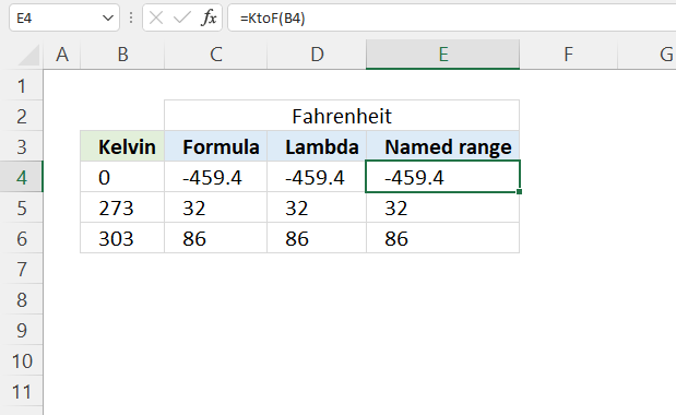
Section 3 below demonstrates how to create a custom function using the LAMBDA function that converts Kelvin to Fahrenheit. It is then named KtoF in the "Name Manager" which allows the user to pass values to the custom function like this: =KtoF(B4) where B4 is a cell reference to cell B4. The use of custom functions makes it easier to reuse complex formulas across worksheets. By creating a custom function, you can encapsulate a complex calculation or series of steps into a single, reusable custom function. This allows you to apply the same logic repeatedly without having to retype or copy-paste the entire formula each time.
What is VBA?
VBA stands for Visual Basic for Applications and is a programming language that is integrated into Microsoft Excel and other Office applications. It allows users to automate tasks, create custom functions, and build sophisticated applications within the Excel environment.
- Automating repetitive tasks, such as data entry, formatting, or report generation.
- Creating macros to record and replay a series of actions for beginners.
- Developing user-defined functions that can be used in Excel formulas. Extending the built-in functionality of Excel.
- Building custom dialog boxes, forms, and user interfaces to interact with data and perform specific tasks.
- Performing complex data analysis, manipulation, and transformation tasks. Automating data import, export, and processing workflows.
- Generating dynamic reports, charts, and dashboards. Automating the creation and distribution of reports.
- Creating standalone Excel-based applications with custom features and functionality.Developing add-ins or plugins that extend the capabilities of Excel.
This all sounds amazing, however, there are a few downsides as well. Sharing VBA-based solutions with users who don't have the necessary permissions or software can be challenging. VBA code can potentially be used to run malicious scripts or macros, posing a security risk if the code is not properly vetted and secured. Some organizations may have strict policies or restrictions on the use of VBA in Excel due to security concerns. This is where LAMBDA function may be used when VBA is not available because of security policies.
Why is the LAMBDA custom function only available in my workbook?
You can export a LAMBDA function to other workbooks, here is how:
Copy a Blank Sheet: One straightforward approach is to copy a blank sheet from the workbook containing the LAMBDA functions to the new workbook. This method transfers all the LAMBDA functions along with the sheet.
What is a recursive Excel formula?
Recursive Excel formulas refer to formulas that reference themselves within their own calculation. In other words, a recursive formula calls itself as part of its own evaluation.
2. Syntax
LAMBDA([parameter1, parameter2, …,] calculation)
| parameter1 | Optional. A value that you want to use in the custom function, you are allowed to use a cell reference, string, or number. Up to 253 parameters. |
| calculation | Required. A formula to evaluate. Must be the last argument, a result is also required. |
3. Example 1

This example demonstrates how to build a custom LAMBDA function, there are three main steps.
- Create a formula.
- Build the LAMBDA function.
- Name the LAMBDA function.
We are going to build a custom LAMBDA function that converts Kelvin to Fahrenheit, it is a simple calculation and works great as a demonstration.
3.1 Create a formula
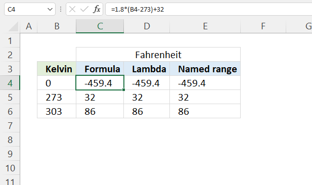
This example shows how to convert Kelvin to Fahrenheit.
This example shows how to convert Kelvin to Fahrenheit, which can be useful when working with temperature measurements in different scientific or engineering contexts. Being able to convert between these scales allows for better collaboration, data sharing, and understanding across disciplines. This conversion is particularly useful when working with temperature data that originates from sources using the Kelvin scale, such as in physics, chemistry, or astronomy, and needs to be expressed in the more commonly used Fahrenheit scale.
The math formula is: F = 1.8(K - 273.15) + 32
F - Fahrenheit which is a temperature scale named after the German physicist Daniel Gabriel Fahrenheit.
K - Kelvin which is the base unit of temperature in the International System of Units (SI).
Formula in cell C4:
Explaining formula
Step 1 - Subtract Kelvin with 273
The minus operator lets you subtract numbers in an Excel formula.
B4-273
0-273 equals -273
Step 2 - Multiply by 1.8
The asterisk character lets you multiply numbers in an Excel formula. The parentheses allow you to control the order of operation.
1.8*(B4-273)
becomes
1.8*-273 equals -491.4
Step 3 - Add 32
The plus operator lets you add numbers in an Excel formula.
1.8*(B4-273)+32
becomes
-491.4 + 32 equals -459.4
3.2 Build the LAMBDA function
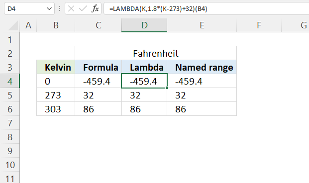
The LAMBDA function has the following syntax: LAMBDA([parameter1, parameter2, …,] calculation)
Formula in cell D4:
The (B4) at the end of the formula is the argument being passed to the custom function. So, when you call this formula, it will take the value in cell B4, plug it into the custom function as the K argument, and return the corresponding temperature in Fahrenheit.
Explaining formula
Step 1 - Formula
This is the formula we built in section 3.1 There is only one input value in this formula.
1.8*(B4-273)+32
Step 2 - LAMBDA function
The LAMBDA function has up to 253 parameters, however, we need only one parameter, in this example named K.
LAMBDA([parameter1, parameter2, …,] calculation)
LAMBDA(K, 1.8*(K-273)+32)
The bolded part above is the formula we built in section 3.1, cell reference B4 is replaced with parameter K.
Step 3 - Pass a value to the LAMBDA function
The LAMBDA function uses parentheses to pass values to the LAMBDA formula.
LAMBDA(K,1.8*(K-273)+32)(B4)
The parameters must be in the same order as you specified them, in this case, it doesn't matter. There is only one parameter.
3.3 Name the LAMBDA function

Excel feature "Named ranges" allows us to assign a custom name to the LAMBDA function. I named it KtoF, shown in cell E4 in the image above.
Formula in cell E4:
Here is how to assign a name to a LAMBDA function:
- Go to tab "Formulas" on the ribbon.
- Press with left mouse button on "Name Manager" button. A dialog box appears.
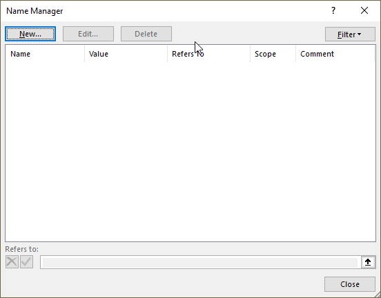
- Press with left mouse button on "New.." button. Another dialog box appears.
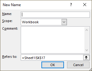
- Type a name.
- Paste the LAMBDA function to "Refers to:" field.
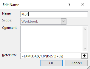
- Press with left mouse button on the "OK" button.
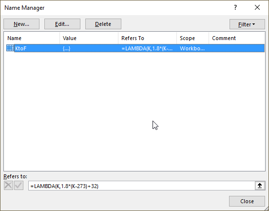
- Press with left mouse button on the "Close" button.
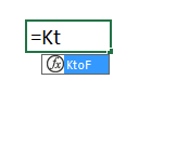
The function we created appears if we type the first characters in the function name in a cell.
4. Analyze word frequency in a cell range
This article demonstrates two ways to calculate the number of times each word appears in a given range of cells. Excel 365 has many new functions that are really useful, I am using the REDUCE function combined with the LAMBDA and VSTACK functions here.
You can also use the TEXTJOIN and the TEXTSPLIT functions, however, they have a limit of 32 767 characters which the REDUCE function doesn't have.
This article also shows a user defined function (UDF) that will work for most Excel versions.
Table of Contents
- How to calculate word frequency in a given cell range - Excel 365 LAMBDA function
- How to calculate word frequency in a given cell range - User defined function
4.1. How to calculate word frequency in a given cell range - Excel 365 LAMBDA function
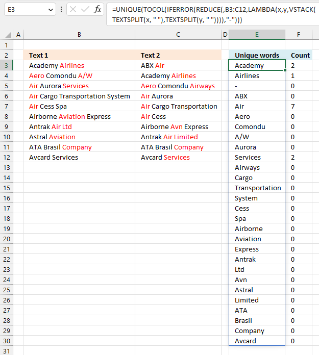
Excel 365 formula in cell E3:
Formula in cell F3:
The formula in cell F3 is explained here: Count how many times a string exists in a cell range (case insensitive)
Explaining the formula in cell E3
Step 1 - Split string based on a space character
The TEXTSPLIT function splits a string into an array based on delimiting values.
Function syntax: TEXTSPLIT(Input_Text, col_delimiter, [row_delimiter], [Ignore_Empty])
TEXTSPLIT(x, " ")
Step 2 - Stack arrays vertically
The VSTACK function combines cell ranges or arrays. Joins data to the first blank cell at the bottom of a cell range or array (vertical stacking)
Function syntax: VSTACK(array1,[array2],...)
VSTACK(TEXTSPLIT(x, " "),TEXTSPLIT(y, " "))
Step 3 - Build the LAMBDA function
The LAMBDA function build custom functions without VBA, macros or javascript.
Function syntax: LAMBDA([parameter1, parameter2, …,] calculation)
LAMBDA(x,y,VSTACK(TEXTSPLIT(x, " "),TEXTSPLIT(y, " ")))
Step 4 - Iterate through each cell in cell range B3:C12
The REDUCE function shrinks an array to an accumulated value, a LAMBDA function is needed to properly accumulate each value in order to return a total.
Function syntax: REDUCE([initial_value], array, lambda(accumulator, value))
REDUCE(,B3:C12,LAMBDA(x,y,VSTACK(TEXTSPLIT(x, " "),TEXTSPLIT(y, " "))))
Step 5 - Replace errors with -
The IFERROR function if the value argument returns an error, the value_if_error argument is used. If the value argument does NOT return an error, the IFERROR function returns the value argument.
Function syntax: IFERROR(value, value_if_error)
IFERROR(REDUCE(,B3:C12,LAMBDA(x,y,VSTACK(TEXTSPLIT(x, " "),TEXTSPLIT(y, " ")))),"-")
Step 6 - Rearrange array to a single column layout
The TOCOL function rearranges values in 2D cell ranges to a single column.
Function syntax: TOCOL(array, [ignore], [scan_by_col])
TOCOL(IFERROR(REDUCE(,B3:C12,LAMBDA(x,y,VSTACK(TEXTSPLIT(x, " "),TEXTSPLIT(y, " ")))),"-"))
Step 7 - Extract unique distinct values from the array
The UNIQUE function returns a unique or unique distinct list.
Function syntax: UNIQUE(array,[by_col],[exactly_once])
UNIQUE(TOCOL(IFERROR(REDUCE(,B3:C12,LAMBDA(x,y,VSTACK(TEXTSPLIT(x, " "),TEXTSPLIT(y, " ")))),"-")))
4.2. How to calculate word frequency in a given cell range - UDF
This user defined function creates a unique distinct list of words and how many times they occur in the selected range.
4.2.1 User defined Function Syntax
FREQWORDS(cell_range, position)
4.2.2 Arguments
| cell_range | Required. The range you want to use. |
| position | Required. Which column to return. The first column contains the values and the second column contains their corresponding frequency. |
4.2.3 Example
Array formula in cell E3:E30:
Array formula in cell F3:F30:
How to create an array formula
4.2.4 VBA
'Name function and declare arguments
Function FreqWords(tbl_array As Range, pos As Integer) As Variant()

'Declare variables and their data types
Dim cell As Variant, wrds As Variant, i As Integer
Dim a As Integer, j As Integer
Dim tmp() As String, nr() As Integer

'Redimension variable tmp so it can grow using Redim Preserve
ReDim tmp(0), nr(0)

'Assign 1 to first value in array variable nr
nr(0) = 1

'Iterate through cells in cell range
For Each cell In tbl_array

  'Split words in cell
  wrds = Split(cell)

  'Iterate thorugh words
  For i = 0 To UBound(wrds)

    'Iterate through arrayvariable tmp
    For j = 0 To UBound(tmp)

      'If variable wrds equal variable tmp then increase value in variable nr by 1
      If wrds(i) = tmp(j) Then
        nr(j) = nr(j) + 1
        a = 1
        Exit For
      End If
    Next j

    'Check if a is not equal to 1
    If a <> 1 Then
      'Copy value from variable wrds to tmp
      tmp(UBound(tmp)) = wrds(i)

      'Add another container to array variable tmp
      ReDim Preserve tmp(UBound(tmp) + 1)
      ReDim Preserve nr(UBound(tmp))
      nr(UBound(tmp)) = 1
    End If
    a = 0
  Next i
Next cell

'Return values in column 1 if argument pos is equal to 1
If pos = 1 Then
  ReDim Preserve tmp(UBound(tmp) - 1)
  FreqWords = Application.Transpose(tmp)
Else

  'Return values in column 2 if argument pos is not equal to 1
  ReDim Preserve nr(UBound(nr) - 1)
  FreqWords = Application.Transpose(nr)
End If
End Function
4.2.5 How to add the User defined Function to your workbook
- Press Alt-F11 to open visual basic editor
- Press with left mouse button on Module on the Insert menu
- Copy and paste vba code
- Exit visual basic editor
5. Multiply numbers in each row by entire cell range
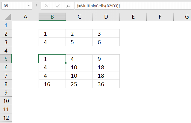
This section demonstrates a recursive LAMBDA function and a User Defined Function (UDF) that multiplies numbers in each row with the remaining rows in a cell range.
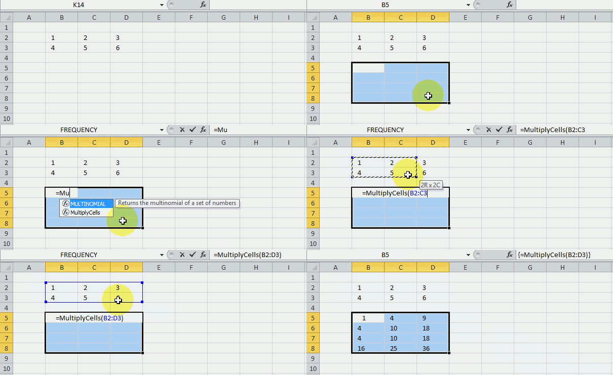
The image above demonstrates the UDF in cell range B5:D8, it takes the first row and multiplies the numbers with all rows in the same cell range. It then continues to the second row and multiplies that row with all rows in the cell range.
Hello Oscar,I have an Excel dataset consisting of 500 rows by 7 columns. I need to generate additional data points from this dataset.I want to multiply (or other function) each row by all 500 rows, creating 250,000 new rows of data.Each cell needs to function as a constant that is multiplied by all the other cells in the same column (which are not acting as constants).How do I do this efficiently? Thanks in advance!
What's on this section
- Multiply cells - recursive LAMBDA function
- MultiplyCells - User Defined Function
5.1. Multiply cells - recursive LAMBDA function
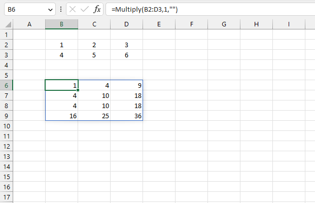
The image above shows the result of a recursive LAMBDA formula in cell B6 that multiplies each row by all rows in the given cell range, read the question here.
A cell range containing 2 rows returns 4 rows. A cell range with 3 rows returns 9 rows, and so on.
Excel 365 formula in cell B6:
Recursive LAMBDA formula:
5.1.1 How to create a named range
- Go to the tab "Formulas" on the ribbon.
- Press the left mouse button on "Name manager". A dialog box appears.
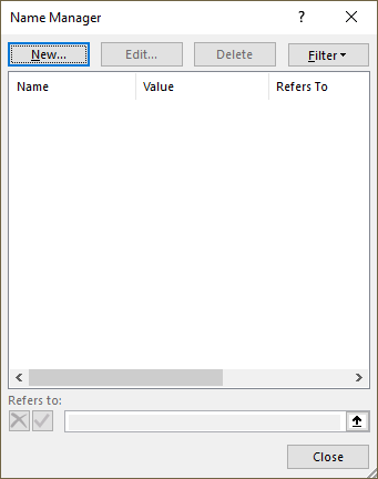
- Press the left mouse button on the "New..." button, see the image above.
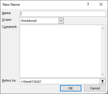
- Name the formula "Multiply".
- Copy/Paste the formula to the "Referes to:" field.
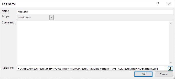
- Press the left mouse button on the "OK" button.
5.1.2 Explaining recursive lambda formula
LAMBDA(rng,n,result,IF(n=(ROWS(rng)+1),DROP(result,1),Multiply(rng,n+1,VSTACK(result,rng*INDEX(rng,n,0)))))
Step 1 - Get row by row from cell range rng
The INDEX function returns a value or reference from a cell range or array, you specify which value based on a row and column number.
Function syntax: INDEX(array, [row_num], [column_num])
INDEX(rng,n,0)
becomes
INDEX({1,2,3;4,5,6},1,0)
and returns
{1,2,3} for the first row.
Step 2 - Multiply rng by the row
The asterisk lets you multiply numbers in an Excel formula.
rng*INDEX(rng,n,0)
becomes
{1,2,3;4,5,6}*{1,2,3}
equals
{1,4,9;4,10,18}.
The next iteration becomes
{1,2,3;4,5,6}*{4,5,6}
and returns
{4,10,18;16,25,36}
Step 3 - Add calculation to result
The VSTACK function combines cell ranges or arrays. Joins data to the first blank cell at the bottom of a cell range or array (vertical stacking)
Function syntax: VSTACK(array1,[array2],...)
VSTACK(result,rng*INDEX(rng,n,0))
becomes
VSTACK("",{1,4,9;4,10,18})
and returns
{"",#N/A,#N/A;1,4,9;4,10,18}.
The next iteration becomes
VSTACK({"",#N/A,#N/A;1,4,9;4,10,18},{4,10,18;16,25,36})
and returns
{"",#N/A,#N/A;1,4,9;4,10,18;4,10,18;16,25,36}
Step 4 - Count rows in range rng
The ROWS function calculate the number of rows in a cell range.
Function syntax: ROWS(array)
ROWS(rng)+1
returns 3.
Step 5 - Delete first row in array
The DROP function removes a given number of rows or columns from a 2D cell range or array.
Function syntax: DROP(array, rows, [columns])
DROP(result,1)
becomes
DROP({"",#N/A,#N/A;1,4,9;4,10,18;4,10,18;16,25,36},1)
and returns
{1,4,9;4,10,18;4,10,18;16,25,36}
Step 6 - Return the result except the first row if n = rows in range rng
The IF function returns one value if the logical test is TRUE and another value if the logical test is FALSE.
Function syntax: IF(logical_test, [value_if_true], [value_if_false])
IF(n=(ROWS(rng)+1),DROP(result,1),Multiply(rng,n+1,VSTACK(result,rng*INDEX(rng,n,0))))
Step 7 - Build LAMBDA function
The LAMBDA function build custom functions without VBA, macros or javascript.
Function syntax: LAMBDA([parameter1, parameter2, …,] calculation)
LAMBDA(rng,n,result,IF(n=(ROWS(rng)+1),DROP(result,1),Multiply(rng,n+1,VSTACK(result,rng*INDEX(rng,n,0)))))
5.1.3 Get Excel *.xlsx file
5.2. MultiplyCells - User Defined Function
Below is a User Defined function I made, it multiplies each row by all other rows in the specified range.
The picture above shows you the UDF using values in cell range B2:B3 and returns the calculated values to cell range B5:D8.
This is a UDF (custom function), you need to copy code to the code module before you can use it.
UDF syntax
Arguments
There is only one argument in this UDF.
range - Cell range
5.2.2. VBA Code
'Name User Defined Function and dimension parameters
Function MultiplyCells(rng As Range)

'Dimension variables and declare data types
Dim rng1 As Variant
Dim tbl() As Variant
Dim rr As Single, r As Single, c As Single, tr As Single

'Save values in range object rng to array variable rng1
rng1 = rng.Value

'Redimension array variable tbl based on rows and columns in range object rng
ReDim tbl(1 To rng.Cells.Rows.CountLarge ^ 2, 1 To rng.Cells.Columns.CountLarge)
tr = 1

'For ... Next statements
For rr = LBound(rng1, 1) To UBound(rng1, 1)
For r = LBound(rng1, 1) To UBound(rng1, 1)
For c = LBound(rng1, 2) To UBound(rng1, 2)

'Multiply values and save the product to array variable tbl
tbl(tr, c) = rng1(rr, c) * rng1(r, c)
Next c

'Add 1 to variable tr and save to variable tr
tr = tr + 1
Next r
Next rr

'Return numbers in array variable tbl to worksheet
MultiplyCells = tbl
End Function
5.2.3. How to enter the UDF as an array formula
Enter this UDF as an array formula, if the range has 2 rows and 3 columns enter the UDF in a cell range with 4 (2*2) rows and 3 columns.
Here are the steps to enter this UDF as an array formula:
- Select cell range B5:D8.
- Type the UDF name and argument:
=MultiplyCells(B2:D3)
- Press and hold CTRL + SHIFT simultaneously.
- Press Enter once.
- Release all keys.
If you did it right the formula now has a curly bracket before and after. Like this {=MultiplyCells(B2:D3)}. Don't enter these yourself. If you are unsure, watch the formula bar carefully in the animated picture above.
5.2.4. Where to put the code?
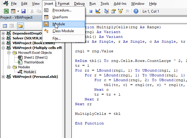
- Press Alt+ F11 to open the Visual Basic Editor (VBE).
- Press with mouse on "Insert" on the top menu, see the image above.
- Press with mouse on "Module" to insert a module to your workbook.
- Copy VBA code above.
- Paste to code window, see the image above.
- Exit VBE and return to Excel.
Copy the following code to a module. How to insert a module to a workbook.
5.2.5. Explaining VBA code
The code explained here is located in the code module. You can find the code module in the VB Editor, press Alt+F11 to open the VB Editor. Press with left mouse button on "Module" found in project explorer.
Function name and arguments
A User Defined Function always starts with "Function" and then a name. This UDF has only one argument. Variable rng is a range object, read more about Defining data types.
Function MultiplyCells(rng As Range)
Declaring variables
tbl() is an array and a variant variable, tbl has two parentheses meaning it is an array. rng1 is also a variant. rr, r, c, and tr are Single variables. Read more about Defining data types.
Dim rng1 As Variant
Dim tbl() As Variant
Dim rr As Single, r As Single, c As Single, tr As Single
Save values from rng (range object) to rng1 (variant)
This speeds up the function considerably if you are working with large cell ranges. Excel copies all the values from the sheet and puts them in memory (array).
rng1 = rng.Value
Build array
ReDim dimensions the tbl array variant, it has the number of rows of the range argument with the power of 2. The values in the array are numbered from 1 to n. There are as many columns as in the range argument.
ReDimtbl(1 To rng.Cells.Rows.CountLarge ^ 2, 1 Torng.Cells.Columns.CountLarge)
Use variables r and c to save values in array
Variable tr keeps track of where to save the next column values in tbl.
tr = 1
For ... Next statement
Repeats a group of statements a specified number of times, here we want to multiply each row by all rows.
For rr = LBound(rng1, 1) To UBound(rng1, 1)
For r = LBound(rng1, 1) To UBound(rng1, 1)
For c = LBound(rng1, 2) To UBound(rng1, 2)
Save value to tbl array
The variables tr, c, rr, and r help us keep track of which values to use and where to save.
tbl(tr, c) = rng1(rr, c) * rng1(r, c)
Add 1 to variable tr
tr = tr + 1
Return tbl values to function
MultiplyCells = tbl
End udf
A function procedure ends with this statement.
End Function
6. Function not working
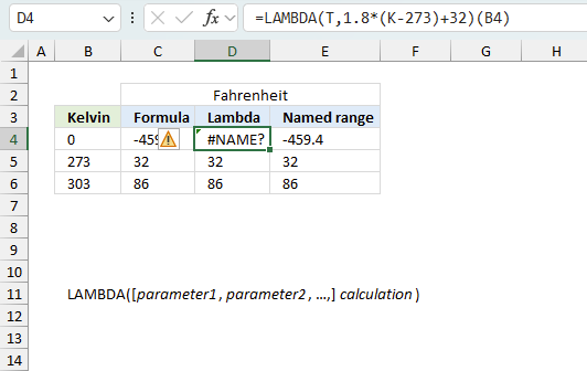
The LAMBDA function returns
- #CALC! error if the input value is missing.
- #NAME? error if you misspell the function name or the variable name is wrong.
- propagates errors, meaning that if the input contains an error (e.g., #VALUE!, #REF!), the function will return the same error.
6.1 Troubleshooting the error value
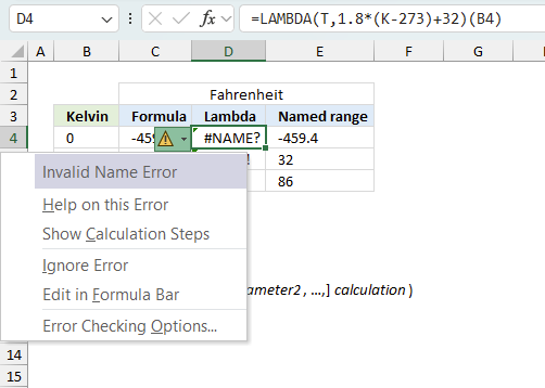
When you encounter an error value in a cell a warning symbol appears, displayed in the image above. Press with mouse on it to see a pop-up menu that lets you get more information about the error.
- The first line describes the error if you press with left mouse button on it.
- The second line opens a pane that explains the error in greater detail.
- The third line takes you to the "Evaluate Formula" tool, a dialog box appears allowing you to examine the formula in greater detail.
- This line lets you ignore the error value meaning the warning icon disappears, however, the error is still in the cell.
- The fifth line lets you edit the formula in the Formula bar.
- The sixth line opens the Excel settings so you can adjust the Error Checking Options.
Here are a few of the most common Excel errors you may encounter.
#NULL error - This error occurs most often if you by mistake use a space character in a formula where it shouldn't be. Excel interprets a space character as an intersection operator. If the ranges don't intersect an #NULL error is returned. The #NULL! error occurs when a formula attempts to calculate the intersection of two ranges that do not actually intersect. This can happen when the wrong range operator is used in the formula, or when the intersection operator (represented by a space character) is used between two ranges that do not overlap. To fix this error double check that the ranges referenced in the formula that use the intersection operator actually have cells in common.
#SPILL error - The #SPILL! error occurs only in version Excel 365 and is caused by a dynamic array being to large, meaning there are cells below and/or to the right that are not empty. This prevents the dynamic array formula expanding into new empty cells.
#DIV/0 error - This error happens if you try to divide a number by 0 (zero) or a value that equates to zero which is not possible mathematically.
#VALUE error - The #VALUE error occurs when a formula has a value that is of the wrong data type. Such as text where a number is expected or when dates are evaluated as text.
#REF error - The #REF error happens when a cell reference is invalid. This can happen if a cell is deleted that is referenced by a formula.
#NAME error - The #NAME error happens if you misspelled a function or a named range.
#NUM error - The #NUM error shows up when you try to use invalid numeric values in formulas, like square root of a negative number.
#N/A error - The #N/A error happens when a value is not available for a formula or found in a given cell range, for example in the VLOOKUP or MATCH functions.
#GETTING_DATA error - The #GETTING_DATA error shows while external sources are loading, this can indicate a delay in fetching the data or that the external source is unavailable right now.
6.2 The formula returns an unexpected value
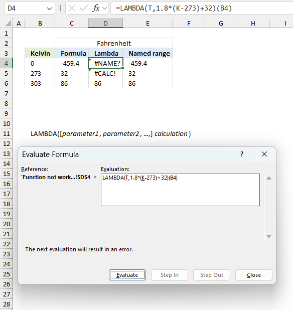
To understand why a formula returns an unexpected value we need to examine the calculations steps in detail. Luckily, Excel has a tool that is really handy in these situations. Here is how to troubleshoot a formula:
- Select the cell containing the formula you want to examine in detail.
- Go to tab “Formulas” on the ribbon.
- Press with left mouse button on "Evaluate Formula" button. A dialog box appears.
The formula appears in a white field inside the dialog box. Underlined expressions are calculations being processed in the next step. The italicized expression is the most recent result. The buttons at the bottom of the dialog box allows you to evaluate the formula in smaller calculations which you control. - Press with left mouse button on the "Evaluate" button located at the bottom of the dialog box to process the underlined expression.
- Repeat pressing the "Evaluate" button until you have seen all calculations step by step. This allows you to examine the formula in greater detail and hopefully find the culprit.
- Press "Close" button to dismiss the dialog box.
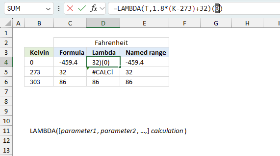
There is also another way to debug formulas using the function key F9. F9 is especially useful if you have a feeling that a specific part of the formula is the issue, this makes it faster than the "Evaluate Formula" tool since you don't need to go through all calculations to find the issue.
- Enter Edit mode: Double-press with left mouse button on the cell or press F2 to enter Edit mode for the formula.
- Select part of the formula: Highlight the specific part of the formula you want to evaluate. You can select and evaluate any part of the formula that could work as a standalone formula.
- Press F9: This will calculate and display the result of just that selected portion.
- Evaluate step-by-step: You can select and evaluate different parts of the formula to see intermediate results.
- Check for errors: This allows you to pinpoint which part of a complex formula may be causing an error.
The image above shows cell reference B4 converted to hard-coded value using the F9 key.
Tips!
- View actual values: Selecting a cell reference and pressing F9 will show the actual values in those cells.
- Exit safely: Press Esc to exit Edit mode without changing the formula. Don't press Enter, as that would replace the formula part with the calculated value.
- Full recalculation: Pressing F9 outside of Edit mode will recalculate all formulas in the workbook.
Remember to be careful not to accidentally overwrite parts of your formula when using F9. Always exit with Esc rather than Enter to preserve the original formula. However, if you make a mistake overwriting the formula it is not the end of the world. You can “undo” the action by pressing keyboard shortcut keys CTRL + z or pressing the “Undo” button
6.3 Other errors
Floating-point arithmetic may give inaccurate results in Excel - Article
Floating-point errors are usually very small, often beyond the 15th decimal place, and in most cases don't affect calculations significantly.
'LAMBDA' function examples
This post explains how to lookup a value and return multiple values. No array formula required.
This article explains how to calculate an overlapping time ranges across multiple days. This can be very useful in situations […]
Table of Contents Count cells containing text from list Count entries based on date and time Count cells with text […]
Functions in 'Logical' category
The LAMBDA function function is one of 16 functions in the 'Logical' category.
Excel function categories
Excel categories
28 Responses to “How to use the LAMBDA function”
Leave a Reply
How to comment
How to add a formula to your comment
<code>Insert your formula here.</code>
Convert less than and larger than signs
Use html character entities instead of less than and larger than signs.
< becomes < and > becomes >
How to add VBA code to your comment
[vb 1="vbnet" language=","]
Put your VBA code here.
[/vb]
How to add a picture to your comment:
Upload picture to postimage.org or imgur
Paste image link to your comment.
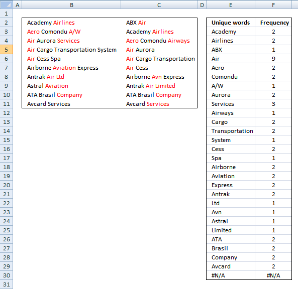




While executing this function,I am facing #value error in the entire column. Please help.
Sam,
This udf is created in excel 2007, what excel version do you have?
Did you remember to enter the second argument?
=FreqWords(B2:C11, 1)
Did you create an array formula?
How to create an array formula
Select cell range E3:E30.
Copy (Ctrl + c) and paste (Ctrl + v) array formula into formula bar.
Press and hold Ctrl + Shift.
Press Enter once.
Release all keys.
Hello Oscar,
first of all MERRY CHRISTMAS AND HAPPY NEW YEAR 2012- also Thank you very much for Word Frequency function.
I would like to ask if it is possible to convert it to a VBA Macro subroutine . I mean is it possible to use Freqwords function with in a sub(). I am novice to programming . please help.
Thank you very much sir.
Srinivas
Hi Oscar
Happy New Year 2012. Thank you very much for Word Frequency UDF. Forget about above request for sub(). I have found alternative.
Thank you
Srinivas
[...] Does this help?.... Excel udf: Word frequency | Get Digital Help - Microsoft Excel resource Example results from the above solution...... [...]
Hi Oscar,
I need your help to find the macro
I have many excel files with multiple sheets and each excel sheet
has many formula which are starting from perticular word e.g. FDS, FDSB, etc some formula has FDS, FDSB occur in the middle of the formula.
i need to find out how many times FDS,FDSB has been appear in the sheet(total count)
below is the formulae for your referance
=FISERROR(FDSB($D21, "IC_ESTIMATE_DATE(ALL, EXP_RPT, QTR, 3, 0, , , 'MM/DD/YYYY')@RC_ESTIMATE_DATE(ALL, EXP_RPT, QTR, +3, 0 , , , 'MM/DD/YYYY')"),"na)
in such a way there are many formulas in all the cells
i just need to count the how many times FDSB occur in one perticular sheet
please help
Best Regards
Rahul Jadhav
Pune
India
Rahul Jadhav,
Have you read this post:
Count multiple text strings in a cell range
Thank you
Rahul Jadhav,
Read this post:
Count text strings in formulas (vba)
Hi Oscar
Thanks for the reply this is what i was looking for thanks once again now i will apply it in all the worksheets.
One more thing i would like to ask is that
How can we identify any protected excel file before opening using macro VBA (e.g. i have a folder with multiple excel files i need to find out using macro how many files are password protected before opening and it should give result on separate workbook.)
is it possible using excel vba macro
Please reply
Best regards
Rahul Jadhav
rahul jadhav,
read this post:
Find out if excel files in a folder are password protected
[…] Rahul Jadhav asks: […]
[…] rahul jadhav asks: […]
Hi Oscar,
Thank you very much for the macro just to infrom you that it is working correctly
Thanks again
Best regards
Rahul Jadhav
Hi Oscar,
Hope you are doing good!!!
My requirement is to copy data from ms excel and paste into ms word on specific position
>Both the files should get open automatically specially ms word
>macro should identify the user define cursor position in ms word file
>then paste the data where user wants to
>In this way i want to copy tables data, text, from excel into ms word on user define posion.
please check and let me know the suitable solution for the same
Have a nice time ahead
Thanking you in advance
Best Regards
Rahul Jdhav
Awesome function!!! Thanks so much for sharing this!
If I understand the question correctly, this function would work:
First you would put your original 500 rows in a table somewhere ("Table1"), and then enter this function as an array (ctrl-shift-enter) starting in cell A1, with seven columns and 250,000 rows. It can be adapted with subtraction from row() and column() if you wish to put your data in a location other than cell A1.
-Alex
Alex,
Great comment!
It works fine, why didn't I think of this.
Your formula is small and genius.
Thank you for commenting.
[…] Excel udf: Word frequency […]
hello oscar,
why u'r formula cannot use in new file?
thanks
boboy,
You need to copy and paste the VBA code to a module in your new file (workbook).
Thank you for that.
The only issue i'm facing is that only the first word of each cell is displaying after entering the formula. Not the full list of each single keyword.
For example, in your spreadsheet, the word "Air" appears 6 times in my list, and the frequency is correct (9).
What am I doing wrong?
Valentino,
you need to enter the formula as an array formula. There are instructions in this article on how to create an array formula.
How do you get the word frequency results in the array to sort by largest to smallest?
Hi great formula!
Quick question - my apologies in advance if it is dumb I typically do not work in Excel.
When I define the array for the results return I am assuming I know the number of unique words I have (in your example you knew there are 27 unique values?). But what happens if I don't know the number of unique words? I selected as an array the whole column but I get many #N/A and then it very inconvenient because I cannot delete these (it tells me I cannot change the array).
Is there a way for it automatically to decide the size of the array?
*I realize supposedly it is a small issue but I am working with a very large file more than 5000 companies that each have many tags and trying to sort the frequency of the tags and it gets messy.
Thanks in advance!
Julie
Is there a way for it automatically to decide the size of the array?
Yes, Excel 365 subscribers don't need to enter this as an array formula. Excel takes care of the output and returns spilled values.
This UDF is for previous Excel versions. It will return blank values if the entered cell range is larger than the number of returned values.
Function FreqWords(tbl_array As Range, pos As Integer) As Variant() Dim cell As Variant, wrds As Variant, i As Integer Dim a As Integer, j As Integer Dim Row As Variant Dim tmp() As String, nr() As Integer ReDim tmp(0), nr(0) nr(0) = 1 For Each cell In tbl_array wrds = Split(cell) For i = 0 To UBound(wrds) For j = 0 To UBound(tmp) If wrds(i) = tmp(j) Then nr(j) = nr(j) + 1 a = 1 Exit For End If Next j If a <> 1 Then tmp(UBound(tmp)) = wrds(i) ReDim Preserve tmp(UBound(tmp) + 1) ReDim Preserve nr(UBound(tmp)) nr(UBound(tmp)) = 1 End If a = 0 Next i Next cell For Row = UBound(tmp) To Application.Caller.Rows.Count tmp(UBound(tmp)) = "" ReDim Preserve tmp(UBound(tmp) + 1) Next Row ReDim Preserve tmp(UBound(tmp) - 1) If pos = 1 Then ReDim Preserve tmp(UBound(tmp) - 1) FreqWords = Application.Transpose(tmp) Else ReDim Preserve nr(UBound(nr) - 1) FreqWords = Application.Transpose(nr) End If End FunctionHi Oscar.
Much like Julie, I mod'ed the formula for a single column, removed the array because I am using Excel 365 and am getting the #NAME? error. I double checked the formula call to the function name and it reads the same. Not sue what else to do...
Michael
Hello again.
Nevermind... just found a thread that suggested adding in the module name infant of the function call, so I renamed the call to Module1.FreqWords and it worked.
Michael