How to use the SUMPRODUCT function
What is the SUMPRODUCT function?
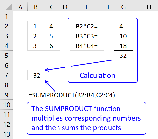
The SUMPRODUCT function calculates the product of corresponding values and then returns the sum of each multiplication.
SUMPRODUCT function example
The picture above shows how the SUMPRODUCT works in greater detail.
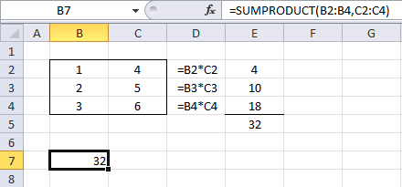
Formula in cell B7:
The SUMPRODUCT function multiplies cell ranges row by row and then adds the numbers and returns a total. The formula in cell B7 multiples values 1*4= 4, 2*5 = 10 and 3*6 =18 and then adds the numbers 4+10+18 equals 32.
Table of Contents
- SUMPRODUCT function syntax
- SUMPRODUCT arguments
- Things to know about the SUMPRODUCT function
- How to use the SUMPRODUCT function
- How to use a logical expression in the SUMPRODUCT function
- How to use multiple conditions in the SUMPRODUCT function
- How to use OR logic in the SUMPRODUCT function
- Sum unique distinct invoices
- Count cells equal to any value in a list
- Count dates inside a date range
- Get Excel *.xlsx file
- Sum based on OR - AND logic
- Find empty cells and sum cells above
1. Excel Function Syntax
SUMPRODUCT(array1, [array2], ...)
2. Arguments
| array1 | Required. Required. The first array argument whose numbers you want to multiply and then sum. |
| [array2] | Optional. Up to 254 additional arguments. |
3. Things to know about the SUMPRODUCT function
The SUMPRODUCT function is one of the most powerful functions in Excel and is one that I often use. I highly recommend learning how it works.
The SUMPRODUCT function requires you to enter it as a regular formula, not an array formula. However, there are exceptions. If you use a logical expression you must enter the formula as an array formula and convert the boolean values to their equivalents.
There are workarounds to this problem which I will demonstrate in the examples below.
4. How to use the SUMPRODUCT function
This example demonstrates how the SUMPRODUCT function works.
Formula in cell B7:
4.1 Explaining formula
Step 1 - Multiplying values on the same row
The first array is in cell range B2:B4 and the second array is in cell range C2:C4.
B2:B4*C2:C4
becomes
{1;2;3} * {4;5;6}
becomes
{1*4; 2*5; 3*6}
and returns {4; 10; 18}.
The same calculations are done in column D and shown in column E, see above picture.
Step 2 - Return the sum of those products
{4; 10; 18}
becomes
4 + 10 + 18
and the function returns 32 in cell B7.
The same calculation is done E5, the sum of the products in cell range E2:E4 is calculated in cell E5. See the above picture.
Now you know the basics. Let's move on to something more interesting.
5. How to use a logical expression in the SUMPRODUCT function
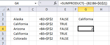
The image above demonstrates a formula in cell G4 that counts how many cells that is equal to the value in cell G2. Note, that this is only an example. I recommend you use the COUNTIF function to count cells based on a condition, it is designed to do that.
Formula in cell G4:
5.1 Explaining formula
Step 1 - Logical expression returns a boolean value that we must convert to numbers
There is only one array in this formula but something else is distorting the picture. A comparison operator (equal sign) and a second cell value (G2) or a comparison value. With these, we have now built a logical expression. This means that the value in cell G2 is compared to all the values in cell range B2:B6 (not case sensitive).
B2:B6=$G$2
becomes
{"Alaska";"California";"Arizona";"California";"Colorado"}="California"
and returns
{FALSE; TRUE; FALSE; TRUE; FALSE}.
They are all boolean values and excel can´t sum these values. We have to convert the values to numerical values. There are a few options, you can:
- Add a zero - (B2:B6=$G$2)+0
- Multiply with 1 - (B2:B6=$G$2)*1
- Double negative signs --(B2:B6=$G$2)
They all convert boolean values to their numerical equivalents. TRUE is 1 and FALSE is 0 (zero).
--( {FALSE;TRUE;FALSE;TRUE;FALSE})
becomes
{0;1;0;1;0}
Step 2 - Return the sum of those products
{0;1;0;1;0}
becomes
0 + 1 + 0 + 1 + 0
and returns 2 in cell G4. There are two cells containing the value "California" in cell range B2:B6.
You accomplish the same thing using the COUNTIF function or count multiple values in different columns using the COUNTIFS function. In fact, you can count entire records in a data set using the COUNTIFS function.
6. How to use multiple conditions in the SUMPRODUCT function
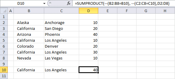
This example shows how to use multiple conditions in the SUMPRODUCT function using AND logic. AND logic means that all conditions must be met on a given row in order to add the number to the total.
Formula in cell D10:
This formula contains three arguments, the SUMPRODUCT function allows you to use up to 30 arguments. You can make the formula somewhat shorter:
This also allows you to have a lot more conditions than 30 if you like and use OR logic if you want. Example 4 demonstrates OR logic.
It is only the available computer memory that is the limit if you use this method. The formula looks like an array formula but no, you are not required to enter it as an array formula.
6.1 Explaining formula
Step 1 - Multiplying corresponding components in the given arrays
The first logical expression B2:B8=B10 uses an equal sign to check if the values in cell range B2:B8 are equal to the value in cell B10.
B2:B8=B10
becomes
{"Alaska";"California";"Arizona";"California";"Colorado";"California";"Nevada"}="California"
and returns
{FALSE; TRUE; FALSE; TRUE; FALSE; TRUE; FALSE}.
The second logical expression is C2:C8=C10, the other logical operators you can use are:
- = equal
- < less than
- > greater than
- <> not equal to
- <= less than or equal to
- >= larger than or equal to
C2:C8=C10
becomes
{"Anchorage";"San Diego";"Phoenix";"Los Angeles";"Denver";"Los Angeles";"Las Vegas"}="Los Angeles"
and returns
{FALSE; FALSE; FALSE; TRUE; FALSE; TRUE; FALSE}.
The third and last logical
(B2:B8=B10)*(C2:C8=C10)*D2:D8
becomes
({FALSE; TRUE; FALSE; TRUE; FALSE; TRUE; FALSE})*({FALSE; FALSE; FALSE; TRUE; FALSE; TRUE; FALSE})*{10; 20; 40; 10; 20; 30; 10}
becomes
{0;0;0;1;0;1;0}*{10; 20; 40; 10; 20; 30; 10}
and returns
{0; 0; 0; 10; 0; 30; 0}
Step 2 - Return the sum of those products
{0; 0; 0; 10; 0; 30; 0}
becomes
10 +30
and returns 40 in cell D10.
7. How to use OR logic in the SUMPRODUCT function

This example shows how to use multiple conditions. A number in cell range D3:D9 is added if the item in cell B12 is found on the corresponding row in cell range B3:B9 OR if the item in C12 is found in cell range C3:C9.
Formula in cell D10:
Explaining formula in cell D10
Step 1 - Compare values to condition
The equal sign lets you compare the condition to values in B3:B9, the result is an array with the same size as B3:B9 containing TRUE or FALSE.
B3:B9=B12
becomes
{"Alaska"; "California"; "Arizona"; "California"; "Colorado"; "California"; "Nevada"}="California"
and returns
{FALSE; TRUE; FALSE; TRUE; FALSE; TRUE; FALSE}.
Step 2 - Compare values to condition
C3:C8=C12
becomes
{"Anchorage"; "San Diego"; "Phoenix"; "Los Angeles"; "Denver"; "Los Angeles"; "Las Vegas"}="Las Vegas"
and returns
{FALSE; FALSE; FALSE; FALSE; FALSE; FALSE; TRUE}.
Step 3 - Apply OR logic
We need to add numbers if at least one of the conditions matches on the same row, this means OR logic.
Mathematical operators between arrays allow you to do more complicated calculations, like this:
* (asterisk) - Both logical expressions must match (AND logic)
+ (plus sign) - Any of the logical expressions must match, it can be all it can be only one. It doesn't matter. (OR logic)
The AND logic behind this is that
- TRUE * TRUE = TRUE (1)
- TRUE * FALSE = FALSE (0)
- FALSE * FALSE = FALSE (0)
The OR logic works like this:
- TRUE + TRUE = TRUE (1)
- TRUE + FALSE = TRUE (1)
- FALSE + FALSE = FALSE (0)
The numbers above show the numerical equivalent of each result. True equals 1 and False equals 0 (zero).
The parentheses shown below let you control the order of calculation, we must do the comparisons before we add the arrays.
(B2:B8=B10)+(C2:C8=C10)
becomes
{FALSE; TRUE; FALSE; TRUE; FALSE; TRUE; FALSE} + {FALSE; FALSE; FALSE; FALSE; FALSE; FALSE; TRUE}
and returns {0; 1; 0; 1; 0; 1; 1}.
Step 4 - Check if result is larger than 0 (zero)
If both values match the conditions the result is two, the result will be twice as much. We can't multiply with two, the larger than character checks if the result is larger than 0 (zero).
((B3:B9=B12)+(C3:C9=C12))>0
becomes
{0; 1; 0; 1; 0; 1; 1}>0
and returns {FALSE; TRUE; FALSE; TRUE; FALSE; TRUE; TRUE}.
Step 5 - Multiply with numbers
((B2:B8=B10)+(C2:C8=C10))*D2:D8
becomes
{FALSE; TRUE; FALSE; TRUE; FALSE; TRUE; TRUE}*D2:D8
becomes
{FALSE; TRUE; FALSE; TRUE; FALSE; TRUE; TRUE}*{10; 20; 40; 10; 20; 30; 10}
and returns {0; 20; 0; 10; 0; 30; 10}.
Step 6 - Add numbers and return total
SUMPRODUCT(((B2:B8=B10)+(C2:C8=C10))*D2:D8)
becomes
SUMPRODUCT({0; 20; 0; 10; 0; 30; 10})
and returns 70.
These expressions check if California is found in cell range B2:B8 or Las Vegas is found in cell range C2:C8. They are found in rows 4, 6,8, and 9.

The SUMPRODUCT function sums the corresponding values in column D and returns 70 in cell D10. 20+10+30+10 equals 70.
8. Sum unique distinct invoices

Question:
I have a long table The key is actually col B&C BUT…sometime there are few rows with same key (like rows 3:4 or rows 8:10). I'd like to sum data in column D and to consider same key rows as one row.
Desired result 216
Can I also add condition that Column E=1 ?
Answer:
I highly recommend a pivot table for this task, it is extremely fast which is good if you have lots of data to work with. This article demonstrates a formula that returns a total based on a condition.

Formula in cell E21:
This formula removes duplicate records and sums values in col D.
Explaining the formula in cell E21
To simplify the explanation I am replacing cell references with named ranges. The formula becomes:
Named Ranges
ColB - $B$3:$B$18
ColC - $C$3:$C$18
ColD - $D$3:$D$18
ColE - $E$3:$E$18
Step 1 - Filter records equal to condition in cell E21
The equal sign lets you compare the values in column E with the condition in cell C21, this is a logical expression and the result is either TRUE or FALSE (boolean values), however, the SUMPRODUCT function can't work with boolean values. We need to convert the TRUE and FALSe to their numerical equivalents. TRUE = 1 and FALSE = 0 (zero).
--(ColE=$C$21)
--({1; 1; 1; 1; 1; 1; 1; 1; 2; 2; 2; 2; 2; 2; 2; 2}=1)
becomes
--({TRUE; TRUE; TRUE; TRUE; TRUE; TRUE; TRUE; TRUE; FALSE; FALSE; FALSE; FALSE; FALSE; FALSE; FALSE; FALSE})
Sumproduct can´t calculate TRUE/FALSE values. Let´s convert values to 1 and 0.
--({TRUE; TRUE; TRUE; TRUE; TRUE; TRUE; TRUE; TRUE; FALSE; FALSE; FALSE; FALSE; FALSE; FALSE; FALSE; FALSE})
becomes
{1; 1; 1; 1; 1; 1; 1; 1; 0; 0; 0; 0; 0; 0; 0; 0}
Step 2 - Create an array with values from col D
ColD
becomes
{5; 5; 100; 55; 47; 9; 9; 9; 4; 4; 100; 55; 47; 9; 9; 9}
Step 3 - Count duplicate records
The COUNTIFS function calculates the number of cells across multiple ranges that equals all given conditions.
1/COUNTIFS(ColB, ColB, ColC, ColC, ColD, ColD, ColE, ColE)
becomes
1/{2; 2; 1; 1; 1; 3; 3; 3; 2; 2; 1; 1; 1; 3; 3; 3}
and returns
{0,5; 0,5; 1; 1; 1; 0,333333333333333; 0,333333333333333; 0,333333333333333; 0,5; 0,5; 1; 1; 1; 0,333333333333333; 0,333333333333333; 0,333333333333333}
Step 4 - Return the sum of the products of the corresponding arrays
=SUMPRODUCT(--(ColE=$C$21), ColD, 1/COUNTIFS(ColB, ColB, ColC, ColC, ColD, ColD, ColE, ColE))
becomes
=SUMPRODUCT({1; 1; 1; 1; 1; 1; 1; 1; 0; 0; 0; 0; 0; 0; 0; 0}, {5; 5; 100; 55; 47; 9; 9; 9; 4; 4; 100; 55; 47; 9; 9; 9}, {0,5; 0,5; 1; 1; 1; 0,333333333333333; 0,333333333333333; 0,333333333333333; 0,5; 0,5; 1; 1; 1; 0,333333333333333; 0,333333333333333; 0,333333333333333})
returns 216 in cell E21.
9. Count cells equal to any value in a list
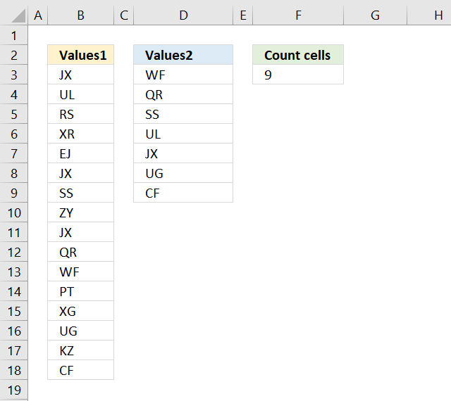
The formula in cell F9 counts the number of cells in column B (Values1) that are equal to any of the values in column D (Values2).
Formula in cell F9:
Explaining formula in cell F9
The COUNTIF function allows you to count cells in a range that are equal to a criterion. The great thing about the COUNTIF function is that it is possible to use criteria.
COUNTIF(B3:B18,D3:D9)
becomes
COUNTIF({"JX"; "UL"; "RS"; "XR"; "EJ"; "JX"; "SS"; "ZY"; "JX"; "QR"; "WF"; "PT"; "XG"; "UG"; "KZ"; "CF"}, {"WF"; "QR"; "SS"; "UL"; "JX"; "UG"; "CF"})
and returns the following array: {1; 1; 1; 1; 3; 1; 1}
The SUMPRODUCT function lets you sum the values in the array without the need to enter the fomula as an array formula.
SUMPRODUCT(COUNTIF(B3:B18,D3:D9))
becomes
SUMPRODUCT({1; 1; 1; 1; 3; 1; 1})
and returns 9 in cell F9. 1+1+1+1+3+1+1 = 9
10. Count dates inside a date range
How do I automatically count dates in a specific date range?

Array formula in cell D3:
This is an array formula so make sure you press Ctrl + Shift + Enter.
Alternative array formula in cell D3:
If you want to count the start date and end date also, try this formula:
Alternative formula:
Explaining alternative formula in cell D3
=SUMPRODUCT(--($A$2:$A$10<=$D$2),--($A$2:$A$10>=$D$1))
Step 1 - Create a boolean array with matching dates to the first criterion
=SUMPRODUCT(--($A$2:$A$10<=$D$2),--($A$2:$A$10>=$D$1))
--($A$2:$A$10<=$D$2)
becomes
--({39448;39450;39448;39474;39459;39473;39453;39452;39463}<=39463)
becomes
--({39448;39450;39448;39474;39459;39473;39453;39452;39463}<=39463)
becomes
--({TRUE;TRUE;TRUE;FALSE;TRUE;FALSE;TRUE;TRUE;TRUE})
becomes
{1;1;1;0;1;0;1;1;1}
Step 2 - Create a boolean array with matching dates to the second criterion
=SUMPRODUCT(--($A$2:$A$10<=$D$2),--($A$2:$A$10>=$D$1))
--($A$2:$A$10>=$D$1)
becomes
--({39448;39450;39448;39474;39459;39473;39453;39452;39463}>=39452)
becomes
--({FALSE;FALSE;FALSE;TRUE;TRUE;TRUE;TRUE;TRUE;TRUE})
becomes
{0;0;0;1;1;1;1;1;1}
Step 3 - All together
=SUMPRODUCT(--($A$2:$A$10<=$D$2),--($A$2:$A$10>=$D$1))
becomes
=SUMPRODUCT({1;1;1;0;1;0;1;1;1},{0;0;0;1;1;1;1;1;1})
becomes
=SUMPRODUCT({0;0;0;0;1;0;1;1;1}) returns 4.
Get Excel *.xls
count-records-between-two-dates-in-excel.xls
Get Excel *.xlsx file
Count cells equal to a value in a list.xlsx
12. Sum based on OR - AND logic
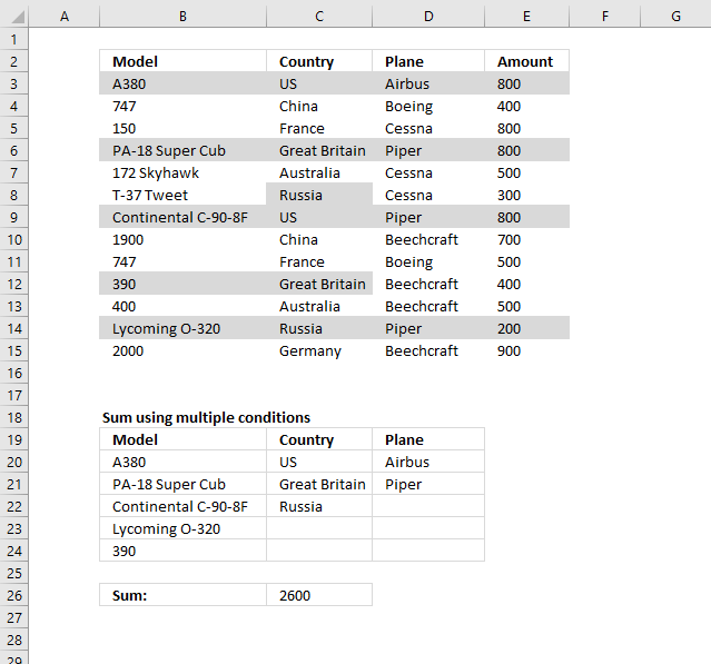
Question:
It's easy to sum a list by multiple criteria, you just use array formula a la: =SUM((column_plane=TRUE)*(column_countries="USA")*(column_producer="Boeing")*(column_to_sum))
But all these are single conditions -- you can't pass multiple conditions, say for example: USA or China or France in column_countries and Airbus or Boeing in column_producer. I know 2 solutions to get around this limitation, but none is perfect:
1) =SUM((column_plane=TRUE)*((column_countries="USA")+(column_countries="China")+(column_countries="France"))* ((column_producer="Airbus") + (column_producer="Boeing"))*(column_to_sum)) -- this one works great, but it's not dinamic at all. What if the user chooses 10 multiple countries or more? You're not gonna write tens of equations for each condition.
2) =SUM((column_countries= IF(TRANSPOSE(contries_selected)=TRUE, TRANSPOSE(countries_selected_names)))*(column_producer="Airbus")*(column_to_sum)) -- that works fine, but this is producing a 2-dimentional matrix and hence is good for one condition only -- notice column_producer has only one value. Now, what if you want to pass multiple values to column_producer as well?
In SQL this equates to
SELECT SUM(column_to_sum)
FROM table
WHERE
(country = "USA" OR country = "France" OR country = "China")
AND
(producer ="Boeing" OR producer="Airbus")
Any idea how to replicate that in Excel???
You can find the question here.
Answer:
The criteria is in B20:D25, I have colored the cells that match. Here is how to avoid writing ten's of equations:
Formula in C26:
Explaining formula in cell C26
Step 1 - Identify criteria B20:B25 in B3:B15
The COUNTIF function counts values based on a condition or criteria. If a match is found 1 is returned and if not found then it returns 0 (zero).
COUNTIF(B20:B25, B3:B15)
becomes
COUNTIF({"A380"; "PA-18 Super Cub"; "Continental C-90-8F"; "Lycoming O-320"; 390; 0},{"A380"; 747; 150; "PA-18 Super Cub"; "172 Skyhawk"; "T-37 Tweet"; "Continental C-90-8F"; 1900; 747; 390; 400; "Lycoming O-320"; 2000})
and returns
{1; 0; 0; 1; 0; 0; 1; 0; 0; 1; 0; 1; 0}
Step 2 - Identify criteria C20:C25 in C3:C15
COUNTIF(C20:C25, C3:C15)
becomes
COUNTIF({"US"; "Great Britain"; "Russia"; 0; 0; 0},{"US"; "China"; "France"; "Great Britain"; "Australia"; "Russia"; "US"; "China"; "France"; "Great Britain"; "Australia"; "Russia"; "Germany"})
and returns
{1; 0; 0; 1; 0; 1; 1; 0; 0; 1; 0; 1; 0}
Step 3 - Identify criteria D20:D25 in D3:D15
COUNTIF(D20:D25,D3:D15)
becomes
COUNTIF({"Airbus"; "Piper"; 0; 0; 0; 0},{"Airbus"; "Boeing"; "Cessna"; "Piper"; "Cessna"; "Cessna"; "Piper"; "Beechcraft"; "Boeing"; "Beechcraft"; "Beechcraft"; "Piper"; "Beechcraft"})
and returns
{1;0;0;1;0;0;1;0;0;0;0;1;0}
Step 4 - Multiply arrays
All conditions must be TRUE in order to return TRUE.
COUNTIF(B20:B25,B3:B15)*COUNTIF(C20:C25,C3:C15)*COUNTIF(D20:D25,D3:D15)
becomes
{1; 0; 0; 1; 0; 0; 1; 0; 0; 1; 0; 1; 0}*{1; 0; 0; 1; 0; 1; 1; 0; 0; 1; 0; 1; 0}*{1;0;0;1;0;0;1;0;0;0;0;1;0}
and returns
{1;0;0;1;0;0;1;0;0;0;0;1;0}
Step 5 - Multiply array with amounts
COUNTIF(B20:B25, B3:B15)*COUNTIF(C20:C25, C3:C15)*COUNTIF(D20:D25, D3:D15)*E3:E15
becomes
{1;0;0;1;0;0;1;0;0;0;0;1;0}*E3:E15
becomes
{1; 0; 0; 1; 0; 0; 1; 0; 0; 0; 0; 1; 0}*{800; 400; 800; 800; 500; 300; 800; 700; 500; 400; 500; 200; 900}
and returns
{800;0;0;800;0;0;800;0;0;0;0;200;0}
Step 6 - Sum array
The SUMPRODUCT function then adds the numbers and returns a total.
SUMPRODUCT(COUNTIF(B20:B25, B3:B15)*COUNTIF(C20:C25, C3:C15)*COUNTIF(D20:D25, D3:D15)*E3:E15)
becomes
SUMPRODUCT({800;0;0;800;0;0;800;0;0;0;0;200;0})
and returns 2600. 800 + 800 + 800 + 200 = 2600.
Get Excel *.xlsx file
pass multiple conditions dynamically.xlsx
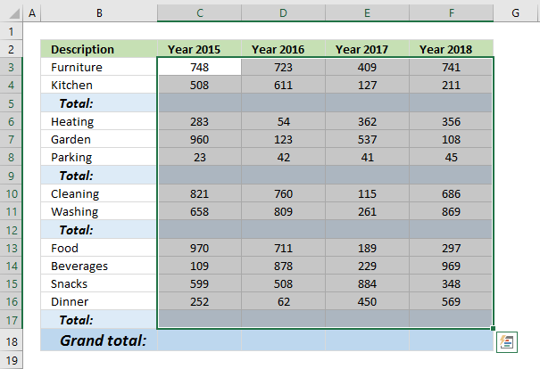
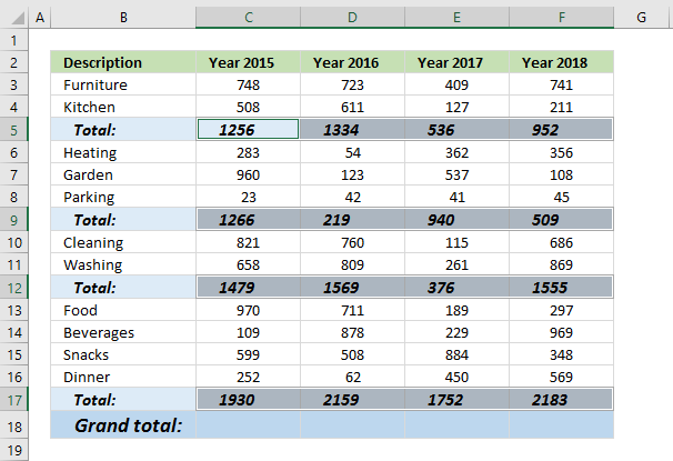
13. Find empty cells and sum cells above
![]()
This article demonstrates how to find empty cells and populate them automatically with a formula that adds numbers above and returns a total.
Is it possible to quickly select all empty cells and then sum cells above to the next empty cell? Yes, I will show you how.
Can I have a formula in grand total (row 18) that only sums all the totals above? Yes!
13.1. How to select empty cells in a cell range
![]()
The image above demonstrates how to find empty cells in a given cell range.
- Select all values and the blank total cells.
- Press F5, a dialog box appears.

- Press the left mouse on the "Special..." button.
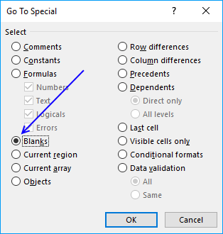
- Press on "Blanks" to select it, then press on the "OK" button.
![]()
13.2. Populate empty cells with a formula
- Go to tab "Home" on the ribbon and press with left mouse button on the "AutoSum" button.
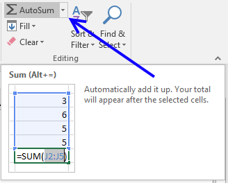
- All empty cells now have a SUM formula that adds all the above values to the next SUM formula.
13.3. Add grand totals that only sums cells populated with formulas
- Select cell C18 and type this formula:
=SUMPRODUCT(ISFORMULA(C3:C17)*C3:C17)
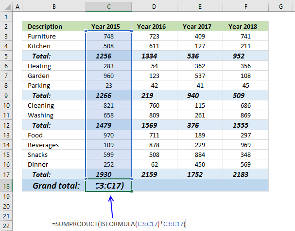
- Press Enter. Copy cell C18 and paste to cell range D18:F18.
13.3.1 Explaining formula in cell C18
Step 1 - Check if cell contains a formula
The ISFORMULA function checks if a cell in cell range C3:C17 has a formula. It returns TRUE or FALSE.
ISFORMULA(C3:C17)
returns this array:
{FALSE; FALSE; TRUE; FALSE; FALSE; FALSE; TRUE; FALSE; FALSE; TRUE; FALSE; FALSE; FALSE; FALSE; TRUE}
The picture below shows this array in column D.
![]()
The array shows that there is a formula in C5, C9, C12, and C17.
Step 2 - Multiply with value
The asterisk character allows you to multiply numbers and boolean values.
ISFORMULA(C3:C17)*C3:C17 multiplies the boolean values with their corresponding values in column C, shown in column E below.
![]()
ISFORMULA(C3:C17)*C3:C17
becomes
{FALSE; FALSE; TRUE; FALSE; FALSE; FALSE; TRUE; FALSE; FALSE; TRUE; FALSE; FALSE; FALSE; FALSE; TRUE}*C3:C17
becomes
{FALSE; FALSE; TRUE; FALSE; FALSE; FALSE; TRUE; FALSE; FALSE; TRUE; FALSE; FALSE; FALSE; FALSE; TRUE}*{748; 508; 1256; 283; 960; 23; 1266; 821; 658; 1479; 970; 109; 599; 252; 1930}
and returns
{0; 0; 1256; 0; 0; 0; 1266; 0; 0; 1479; 0; 0; 0; 0; 1930}
Step 3 - Add values and return the total
The SUMPRODUCT function then sums all values in the array.
SUMPRODUCT(ISFORMULA(C3:C17)*C3:C17)
becomes
SUMPRODUCT({0; 0; 1256; 0; 0; 0; 1266; 0; 0; 1479; 0; 0; 0; 0; 1930})
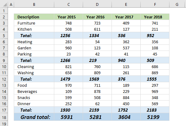
and returns 5931 in cell C18.
Why not use the SUM function? You need to enter it as an array formula if you use the SUM function. Use the SUM function if you are an Excel 365 user.
13.4. Add grand totals that only sums cells populated with formulas - Excel 2013
![]()
The following formula won't work, the SUMIF function seems to not be capable of processing the ISFORMULA function. The ISFORMULA function is an Excel 2013 function, they seem incompatible.
=SUMIF(C3:C17, ISFORMULA(C3:C17))
Let me know if you have a solution that allows me to use the SUMIF function.
13.5. Add grand totals that only sums cells populated with formulas - Excel 365
![]()
=SUM(FILTER(C3:C17, ISFORMULA(C3:C17)))
5.1 Explaining formula
Step 1 - Check if cell contains formula
The ISFORMULA function returns a boolean value TRUE or FALSE if a cell contains a formula or not.
ISFORMULA(C3:C17)
Step 2 - Filter numbers based on boolean values
FILTER(C3:C17,ISFORMULA(C3:C17))
Step 3 - Add numbers and return a total
SUM(FILTER(C3:C17,ISFORMULA(C3:C17)))
Recommended articles
- SUMPRODUCT function (Microsoft Excel)
- SUMPRODUCT function (Xelplus)
- SUMPRODUCT Function (ExcelJet)
'SUMPRODUCT' function examples

This post explains how to lookup a value and return multiple values. No array formula required.
Table of Contents Automate net asset value (NAV) calculation on your stock portfolio Calculate your stock portfolio performance with Net […]
Table of Contents AVERAGE ignore blanks Average - ignore blanks and errors Average - ignore blanks in non-contiguous cells Weighted […]
Functions in 'Math and trigonometry' category
The SUMPRODUCT function function is one of 73 functions in the 'Math and trigonometry' category.
Excel function categories
Excel categories
9 Responses to “How to use the SUMPRODUCT function”
Leave a Reply
How to comment
How to add a formula to your comment
<code>Insert your formula here.</code>
Convert less than and larger than signs
Use html character entities instead of less than and larger than signs.
< becomes < and > becomes >
How to add VBA code to your comment
[vb 1="vbnet" language=","]
Put your VBA code here.
[/vb]
How to add a picture to your comment:
Upload picture to postimage.org or imgur
Paste image link to your comment.
This can be solved without using array in the same fashion (makes the file much lighter when compared to array) =sumproduct((logical test on array1)*(logical test on array2)*...*(result array))
Vipul,
Thanks!
Formula in C26:
=SUMPRODUCT(COUNTIF(B20:B25, Model)*COUNTIF(C20:C25, Country)*COUNTIF(D20:D25, Plane)*Amount) + Enter
Hi Oscar,
While reading this article "How to use excel SUMPRODUCT function" I detected what I think is a minor error.
In example 3 (The California-Los angeles example), you say that the formula transaltes to:
=({FALSE; TRUE; FALSE; TRUE; FALSE; TRUE; FALSE})*({FALSE; FALSE; FALSE; FALSE; FALSE; FALSE; TRUE})*{10; 20; 40; 10; 20; 30; 10}
but i think that the second set of boolean values is not correct and should be:
=({FALSE; TRUE; FALSE; TRUE; FALSE; TRUE; FALSE})*({FALSE; FALSE; FALSE; TRUE; FALSE; TRUE; FALSE})*{10; 20; 40; 10; 20; 30; 10}
Is that correct or I understood incorrectly?
Thanks in advance for your support with this blog.
Regards
Arturo
Arturo,
thanks!!
As alternative solution in cell C18 you can write the formula
=SUM(C3:C17)/2miho66,
Yes, you are right. A lot easier, thanks for commenting.
[…] SUMPRODUCT(array1, array2, ) Returns the sum of the products of the corresponding ranges or arrays […]
Another complete this task:
after use autosum, select again whole range (C3:F17) and use Find&Replace to replace sting "sum(" with "subtotal(9,"
Ciprian Stoian,
Yes, you are right. The SUBTOTAL function ignores other SUBTOTALS to avoid double counting.
Thank you for commenting.